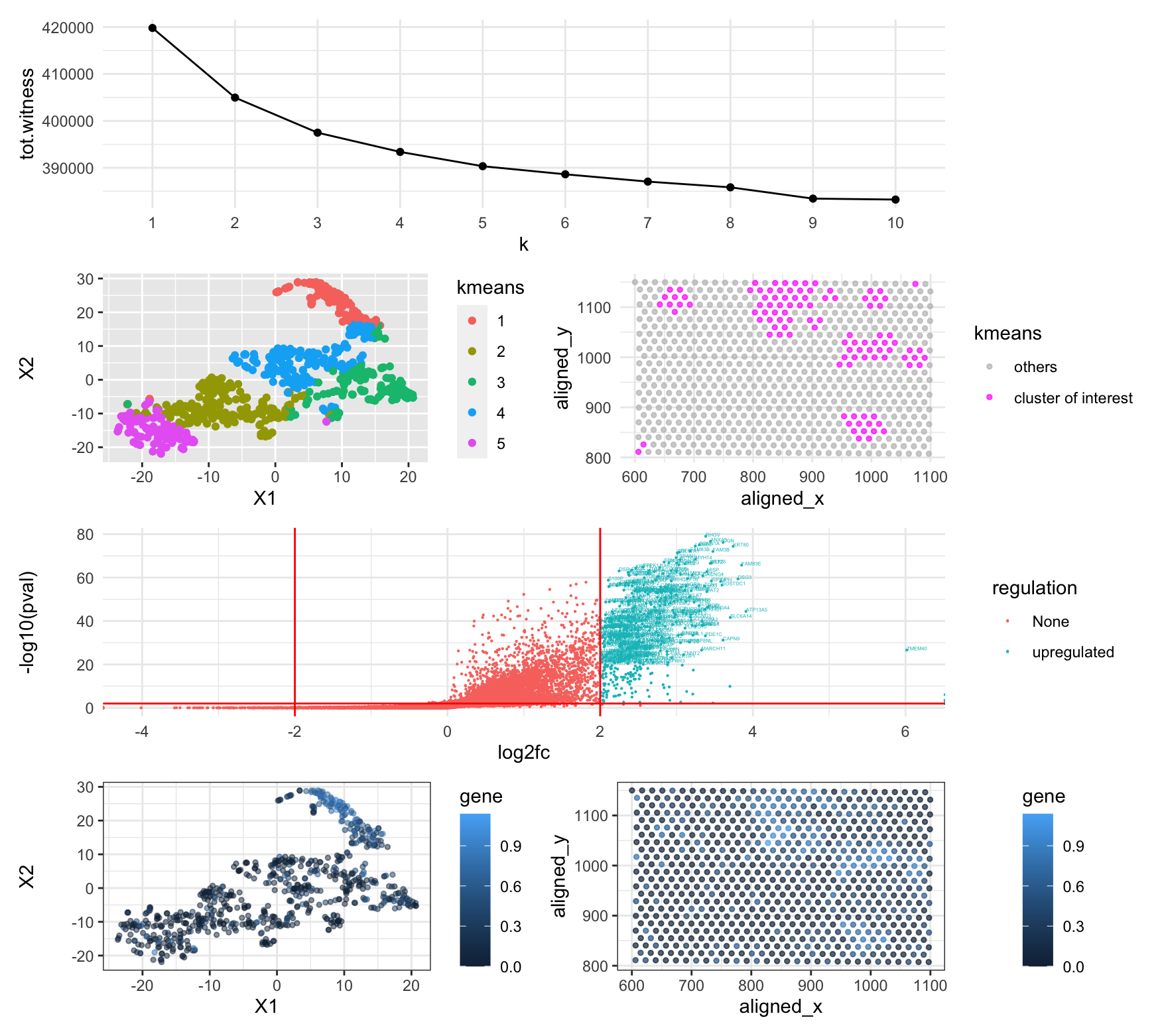
Differentially expressed gene (DSC2) in cell clusters by k-means

Use/adapt your code from HW4 to identify the same cell-type in the other dataset. Create a multi-panel data visualization and write a description to convince me you found the same cell-type.
The very top panel showed an elbow plot to find an optimal k. I found that The k-means methods clustered barcodes based on gene expression levels. I found k=5 could be optimal since the total witness stopped dropping drastically after k=5. I then plotted the k-means clusters in t-SNE (second row left panel). I picked cluster 1 as it This cluster looks a bit scattered in physical space though (second row right panel). After doing Wilcoxon one-sided tests for all genes in cluster 1, I plotted the volcano plot (third row panel) and identified tons of up-regulated genes. ‘DSC2’ (what I picked for hw4) is one of the significantly expressed genes in this cluster based on p-values (<0.01). To visualize the expression level of this gene, I plotted all barcodes again in the t-SNE space labeled by gene expression levels (bottom row left panel) and in physical space (bottom row right panel). We can see that this gene is significantly expressed higher in this cluster. As a result, I think I found the same cell type because the same gene was also significantly expressed higher in the cell cluster picked for hw4.
Write a description of what you changed and why you think you had to change it.
I changed k from 4 (pikachu) to 5 (eevee). I think I may be supposed to use a larger k for the pikachu dataset as my previously chosen cluster could have multiple subtypes. I think there is a lower optimal number of transcriptionally distinct cell-clusters in the spot-based Eevee dataset compared to the single-cell resolution Pikachu dataset because one spot could contain many cells so that the resolution is larger than single-cell. I also plotted the k-means clusters in t-SNE space, where clusters are more salient than cluster in the original space. I am now using a volcano plot to demonstrate p-values so that we can use both the log2FC and p-value thresholds to identify significant up-regulated genes.
Please share the code you used to reproduce this data visualization.
data <- read.csv('eevee.csv.gz', row.names = 1)
library(ggplot2)
library(patchwork)
library(Rtsne)
library(dplyr)

# load and preprocess data
set.seed(0)
pos <- data[, 2:3]
total_count <- rowSums(data[ ,4:ncol(data)], na.rm=TRUE)
gexp <- data[, 4:ncol(data)]
gexpnorm <- log10(gexp/rowSums(gexp) * mean(rowSums(gexp))+1)

# test for total withinness change with k -- find optimal k
tot.witness = c()
for (i in 1:10){
  km <- kmeans(gexpnorm, centers=i)
  tot.witness = append(tot.witness, km$tot.withinss)
}
df.witness = data.frame(k=c(1:10), total.witness=tot.witness)
p00 = ggplot(df.witness, aes(x=k, y=tot.witness)) + geom_line() +
  geom_point() + theme_minimal() + scale_x_discrete(limits=as.factor(c(1:10)))

# plot k-means clusters in PC space
km <- kmeans(gexpnorm, centers=5)
# pca = data.frame(prcomp(gexpnorm)$x[,1:2], kmeans=as.factor(km$cluster))
emb <- Rtsne(prcomp(gexpnorm)$x[,1:20])$Y
df0 = data.frame(emb, kmeans=as.factor(km$cluster))
p2 = ggplot(df0, aes(x=X1, y=X2, col=kmeans),
            size=3) + geom_point()

# plot barcodes clusers based on gene expression in physical space
df <- data.frame(data, kmeans=as.factor(km$cluster == 1))
p0 = ggplot(df) + geom_point(aes(x = aligned_x, y=aligned_y, col=kmeans),
                             size=1, alpha=0.7) + theme_minimal() +
  scale_color_manual(breaks = c('FALSE', 'TRUE'), values=c("gray", "magenta"),
                     labels = c( "others","cluster of interest"))

# pick the most distinct cluster in PC space
results <- sapply(colnames(gexpnorm), function(g) {
  wilcox.test(gexpnorm[km$cluster == 1, g],
              gexpnorm[km$cluster != 1, g],
              alternative = "greater")$p.val})
pval = data.frame(pval = results)
pval$gene = row.names(pval)

# find log2 fold change for each and plot p-values of genes
logfc <- sapply(colnames(gexpnorm), function(i) {
  log2(mean(gexpnorm[km$cluster == 1, i])/mean(gexpnorm[km$cluster != 5, i]))
})
pval$log2fc = logfc

pval = pval %>%
  mutate(regulation = case_when((log2fc>2 & pval<0.01) ~ "upregulated",
                                (log2fc<=2 | pval>=0.01)  ~ "None"))

p3 = ggplot(pval, aes(x=log2fc, y=-log10(pval), col=regulation, label=gene), size=0.5) +
  geom_point() +
  geom_vline(xintercept = 2, col='red') + geom_vline(xintercept = -2, col='red') +
  geom_hline(yintercept = -log10(0.01), col='red') +
  geom_text(aes(label=ifelse(((pval<1e-2)&(log2fc>2)),gene, "")),hjust=0,vjust=0, size=2) +
  theme_minimal()

# plot important genes in t-SNE
df1 = data.frame(emb, gene = gexpnorm[,"DSC2"])
p4 = ggplot(df1) +
  geom_point(aes(x = X1, y = X2, col=gene), size=1, alpha=0.5) +
  theme_bw()

p5 = ggplot(data.frame(data[, 2:3], gene = gexpnorm[,'DSC2'])) +
  geom_point(aes(x=aligned_x, y=aligned_y, col=gene), size=1, alpha=0.7) +
  theme_bw()

p00 / (p2 + p0) / p3 /(p4+p5)
external resources
https://dplyr.tidyverse.org/reference/case_when.html