Identification of Myoepithelial Cells in Breast Cancer Tissue: For Eevee Dataset

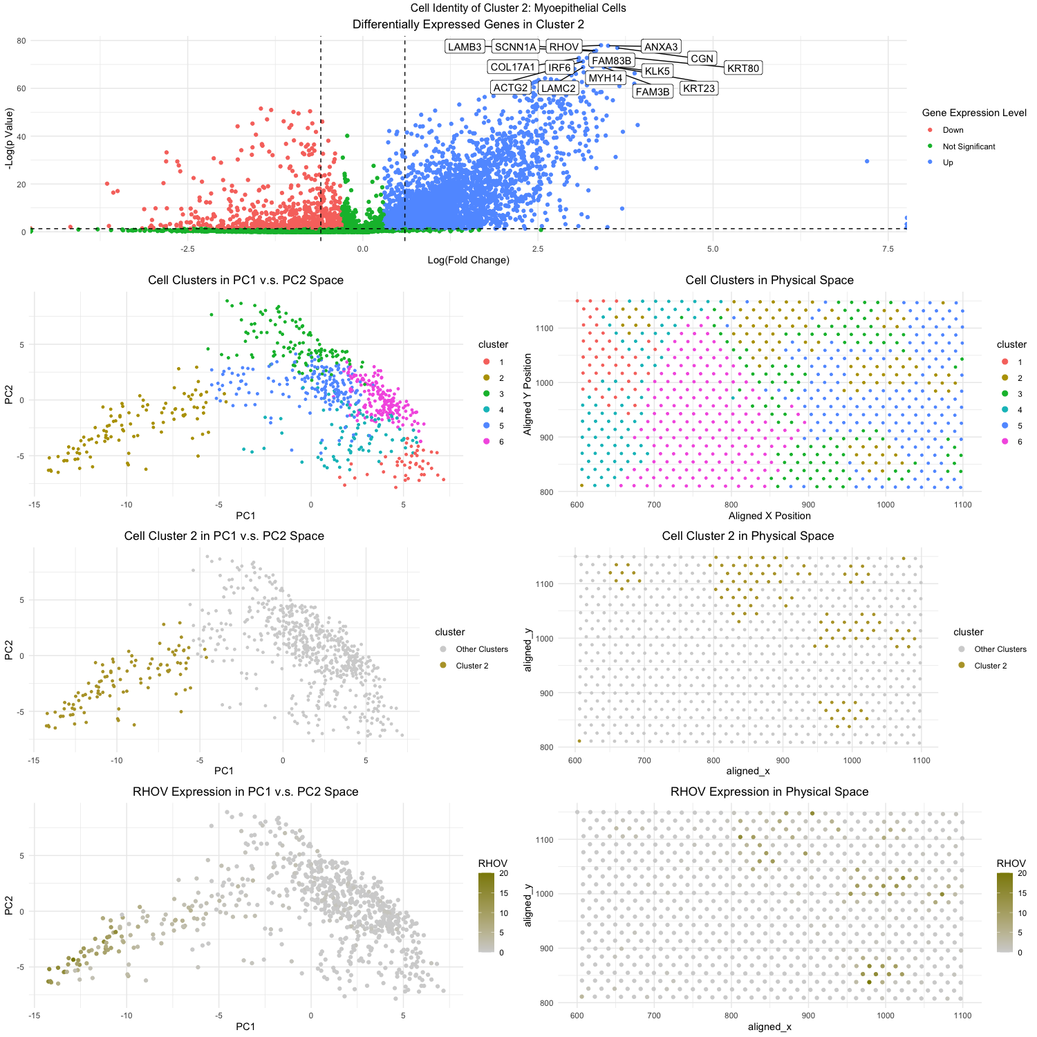
Figure Description:
The workflow from homework 4 was applied with some modifications (as described below) to analyze the eevee dataset and identify a cluster of cells that were of the breast myoepithelial type. This led my analysis to cluster 2, which when looking at the topmost volcano plot, contained the following differentially expressed genes: RHOV, ANXA3, LAMB3, KRT80, and COL17A1. The expression of RHOV can further be visualized as being notably high in cluster 2 when looking at the bottom 2 plots.
Now as to why I am confident that cluster 2 is associated with the breast myoepithelial cell type, we can analyze each of RHOV, ANXA3, LAMB3, KRT80, and COL17A1. Just in 2023, researchers were able to identify RHOV as a pro-metastasis factor for triple-negative breast cancer. For ANXA3, researchers discovered that ANXA3 upregulation triggers mesenchymal-to-epithelial differentiation and is also upregulated in breast cancer samples. LAMB3 and KRT80 has been associated as a pro-metastasis factor for breast cancer and promotes its ability to invade other tissues. And lastly, COL17A1 upregulation has been noted to promote the formation of multilayered, transformed epithelia, which can be an early sign of cancer development. As a final source of evidence as well, if one were to query RHOV, ANXA3, LAMB3, KRT80, and COL17A1 on the protein atlas database (proteinatlas.org), one would note that the highest associated tissue cell type would be breast myoepithelial cells.
Description of Changes Made:
Changes in the workflow involved two aspects: (1) I reduced the number of PCs utilized for k-Means from 10 to 8 and (2) I reduced the number of centers / clusters for k-Means from 10 to 6. The first change was made because I noticed that the scree-plot for the eevee dataset showed that 8 PCs was actually enough to represent nearly all of the significant variance of the dataset. Unlike for the pikachu dataset, where the variance plateaued out to 0 from 10 PCs onward, for the eevee dataset, the variance plateaued to 0 from 8 PCs onward. The second change was made because the elbow plot of total withiness showed that the elbow was actually at k = 6 instead of k = 10. Now, to biologically reason and understand why these changes were necessary, I believe we can look at the difference in the datasets. The pikachu dataset contains 17,135 distinct cells / observations, while the eevee dataset only contains 709 observations. This nearly 95% decrease in observations makes sense if we remember that the pikachu dataset was created on a single-cell level while the eevee dataset was created using spatially-encoded beads that grouped multiple cells together.
With the Eevee dataset, characterized by spatially-encoded beads grouping multiple cells together, the scree plot analysis demonstrated that the significant variance in transcriptional profiles could be effectively represented by just 8 principal components, mirroring the potential reduced cellular resolution and inherent spatial aggregation. Furthermore, the elbow plot for total within-cluster sum of squares revealed that 6 clusters were optimal, reflecting the potential lower level of cellular heterogeneity in the spatially-encoded dataset. In other words, I believe the significantly reduced number of observations opens room for potentially less variance within the dataset, and ultimately less number of distinct groups / clusterings when compared to the pikachu dataset.
Another rather more procedural than technical change involved the selection of the cluster to analyze. Rather than randomly selecting a cluster to analyze, as I had done in homework 4, this time I had to target my search to look for breast myoepithelial cells. Hence, I decided to collect the top 5 genes associated with the breast myoepithelial cell cluster I had analyzed in homework 4 and search for the cluster that had the highest expression of such genes. Such an analysis paid off as this ultimately helped me narrow down my search to cluster 2, which further downstream analysis (as mentioned above) helped me conclude cluster 2 also contained breast myoepithelial cells.
References:
[1] 10.1111/cas.15783
[2] 10.1038/s41419-017-0143-z
[3] 10.1038/s41420-020-00371-2
[4] 10.1038/s41467-019-09676-y
[5] 10.1016/j.cub.2021.04.078
# Load necessary packages
library(factoextra)
library(NbClust)
library(cluster)
library(ggrepel)
library(ggplot2)
library(gridExtra)
library(dplyr)
library(patchwork)

# Load in the data
data <- read.csv("eevee.csv.gz", row.names = 1)
head(data)

pos <- data[,2:3]
gexp <- data[,4:ncol(data)]

# Filter the cells first for meaningful expression
cell_keep <- rownames(gexp)[rowSums(gexp) > 0]
pos <- pos[cell_keep,]
gexp <- gexp[cell_keep,]

# Normalize gene expression
total_gexp <- rowSums(gexp)
norm_gexp <- (gexp/total_gexp) * median(total_gexp)
norm_gexp <- log10(norm_gexp + 1)

# Run PCA test
pcs <- prcomp(norm_gexp)

# Find optimal PCs for kMeans
plot(1:20, pcs$sdev[1:20], type = "l")
plot(1:10, pcs$sdev[1:10], type = "l")

# 8 PCs seem to account pretty much all the meaningful variance of the dataset
opt_pc <- 8

## Set seed for reproducibility of kMeans
set.seed(1)

# Determine optimal number of k's (centroids) for kMeans
elbow <- fviz_nbclust(norm_gexp, kmeans, method = "wss") +
  geom_vline(xintercept = 5, linetype = 2) +
  labs(subtitle = "Elbow Method")

elbow

# Identifying optimal number of k's
opt_k <- 6

# Run kMeans clustering
kmean_cluster <- kmeans(pcs$x[,1:opt_pc], centers = opt_k)
df_cluster <- data.frame(pos, cluster = as.factor(kmean_cluster$cluster), gexp, pcs$x[,1:opt_pc])

# Visualize the clusters in PC1 v.s. PC2
pc_cluster <- ggplot(data = df_cluster, aes(x = PC1, y = PC2, col = cluster)) +
  geom_point(size = 1) +
  theme_minimal() +
  labs(title = "Cell Clusters in PC1 v.s. PC2 Space") +
  theme(plot.title = element_text(hjust = 0.5)) +
  guides(color = guide_legend(override.aes = list(size = 2.5)))

pc_cluster

# Visualize the clusters in physical space
physical_cluster <- ggplot(data = df_cluster, aes(x = aligned_x, y = aligned_y, col = cluster)) +
  geom_point(size = 1) +
  theme_minimal() +
  labs(title = "Cell Clusters in Physical Space", x = "Aligned X Position", y= "Aligned Y Position") +
  theme(plot.title = element_text(hjust = 0.5)) +
  guides(color = guide_legend(override.aes = list(size = 2.5)))

physical_cluster

## The top 5 genes of myoepithelial cells identified prior are in prior_gene_list
prior_gene_list <- list("DSP", "DST", "KRT14", "KRT5", "KRT6B")
for (gene in prior_gene_list) {
  # Check if the gene exists as a column name in df_cluster
  if (gene %in% colnames(df_cluster)) {
    print(gene)
  }
}

## Going to visualize where DSP & DST expression is high
dst_PCA <- ggplot(data = df_cluster, aes(x = PC1, y = PC2, col = DST)) +
  geom_point(size = 1) +
  theme_bw() +
  scale_color_gradient(low = 'lightgrey', high = 'blue') +
  labs(x = "Aligned X Position", y = "Algned Y Position", color = "DST", title = "DST Expression in PCA Space") +
  theme(plot.title = element_text(hjust = 0.5))

dst_PCA

dsp_PCA <- ggplot(data = df_cluster, aes(x = PC1, y = PC2, col = DSP)) +
  geom_point(size = 1) +
  theme_bw() +
  scale_color_gradient(low = 'lightgrey', high = 'blue') +
  labs(x = "Aligned X Position", y = "Algned Y Position", color = "DSP", title = "DSP Expression in PCA Space") +
  theme(plot.title = element_text(hjust = 0.5))

dst_PCA

pc_cluster + dst_PCA + dsp_PCA # Looks like cluster 2

# Pick cluster 2 to analyze

# Visualize cluster 2 in PC1 v.s. PC2
pc_cluster2 <- ggplot(data = df_cluster, aes(x = PC1, y = PC2, col = cluster == 2)) +
  geom_point(size = 1) +
  theme_minimal() +
  labs(title = "Cell Cluster 2 in PC1 v.s. PC2 Space") +
  theme(plot.title = element_text(hjust = 0.5)) +
  guides(color = guide_legend(override.aes = list(size = 2.5))) +
  scale_color_manual(name = "cluster", values = c('lightgrey', '#B6A133'), labels = c("Other Clusters", "Cluster 2"))

pc_cluster2

# Visualize cluster 2 in physical space
physical_cluster2 <- ggplot(data = df_cluster, aes(x = aligned_x, y = aligned_y, col = cluster == 2)) +
  geom_point(size = 1) +
  theme_minimal() +
  labs(title = "Cell Cluster 2 in Physical Space") +
  theme(plot.title = element_text(hjust = 0.5)) +
  guides(color = guide_legend(override.aes = list(size = 2.5))) +
  scale_color_manual(name = "cluster", values = c('lightgrey', '#B6A133'), labels = c("Other Clusters", "Cluster 2"))

physical_cluster2

# Volcano Plot Creation

# Identify cells that are within cluster 2 and not within cluster 2
cluster2_cells <- df_cluster[df_cluster$cluster == 2,]
not_cluster2_cells <- df_cluster[df_cluster$cluster != 2,]

# Use Wilcox test to find differentially expressed genes within cluster 2
diff_genes <- sapply(colnames(gexp), function(g) {
  wilcox.test(norm_gexp[row.names(cluster2_cells), g],
              norm_gexp[row.names(not_cluster2_cells), g])$p.value
})

# Calculate statistics for volcano plot
# ratio for fold change
fc <- sapply(colnames(gexp), function(g) {
  log2( mean(norm_gexp[row.names(cluster2_cells), g])
        / mean(norm_gexp[row.names(not_cluster2_cells), g]))
})

volcano_df <- data.frame(fc, p = ifelse(is.infinite(-log10(diff_genes)), 350, -log10(diff_genes)))

upreg_genes <- sapply(colnames(gexp), function(g) {
  wilcox.test(norm_gexp[row.names(cluster2_cells), g],
              norm_gexp[row.names(not_cluster2_cells), g],
              alternative = 'greater')$p.value
})

top_genes <- sort(upreg_genes, decreasing = FALSE)[1:15]
top_genes

volcano_df$express <- "Not Significant"
volcano_df$express[volcano_df$fc > 0.3 & volcano_df$p > -log10(0.05)] <- "Up"
volcano_df$express[volcano_df$fc < -0.3 & volcano_df$p > -log10(0.05)] <- "Down"

# Now plot the volcano plot
volcano <- ggplot(volcano_df) +
  geom_point(aes(x = fc, y = p, col = express)) +
  geom_hline(yintercept = -log10(0.05), linetype = "dashed") +
  geom_vline(xintercept = c(-0.6, 0.6), linetype = "dashed") +
  geom_label_repel(data = volcano_df[names(top_genes),],
                   aes(x = fc, y = p, label = names(top_genes)),
                   max.overlaps = 40) +
  theme_minimal() +
  labs(title = "Differentially Expressed Genes in Cluster 2", x = "Log(Fold Change)", y = "-Log(p Value)", col = "Gene Expression Level") +
  theme(plot.title = element_text(hjust = 0.5))

volcano

# Plot RHOV (most significant gene)
genePC_plot <- ggplot(data = df_cluster) +
  geom_point(aes(x = PC1, y = PC2, col = RHOV)) +
  theme_minimal() +
  scale_color_gradient(low = "lightgrey", high = "#8B8800") +
  labs(title = "RHOV Expression in PC1 v.s. PC2 Space") +
  theme(plot.title = element_text(hjust = 0.5))

genePC_plot

gene2d_plot <- ggplot(df_cluster) +
  geom_point(aes(x = aligned_x, y = aligned_y, col = RHOV)) +
  theme_minimal() +
  scale_color_gradient(low = "lightgrey", high = "#8B8800") +
  labs(title = "RHOV Expression in Physical Space") +
  theme(plot.title = element_text(hjust = 0.5))

gene2d_plot

## Combine plots together
lay <- rbind(c(1,1),
             c(2,3),
             c(4,5),
             c(6,7))

grid.arrange(volcano,
             pc_cluster, physical_cluster,
             pc_cluster2, physical_cluster2,
             genePC_plot, gene2d_plot,
             layout_matrix = lay,
             top = "Cell Identity of Cluster 2: Myoepithelial Cells")

# References
# Elbow Method in R: https://www.statology.org/elbow-method-in-r/
# Volcano plot was done in conjunction / simiar research with classmate Jonathan