Differential Expression of ERBB2 Gene in Pikachu Data

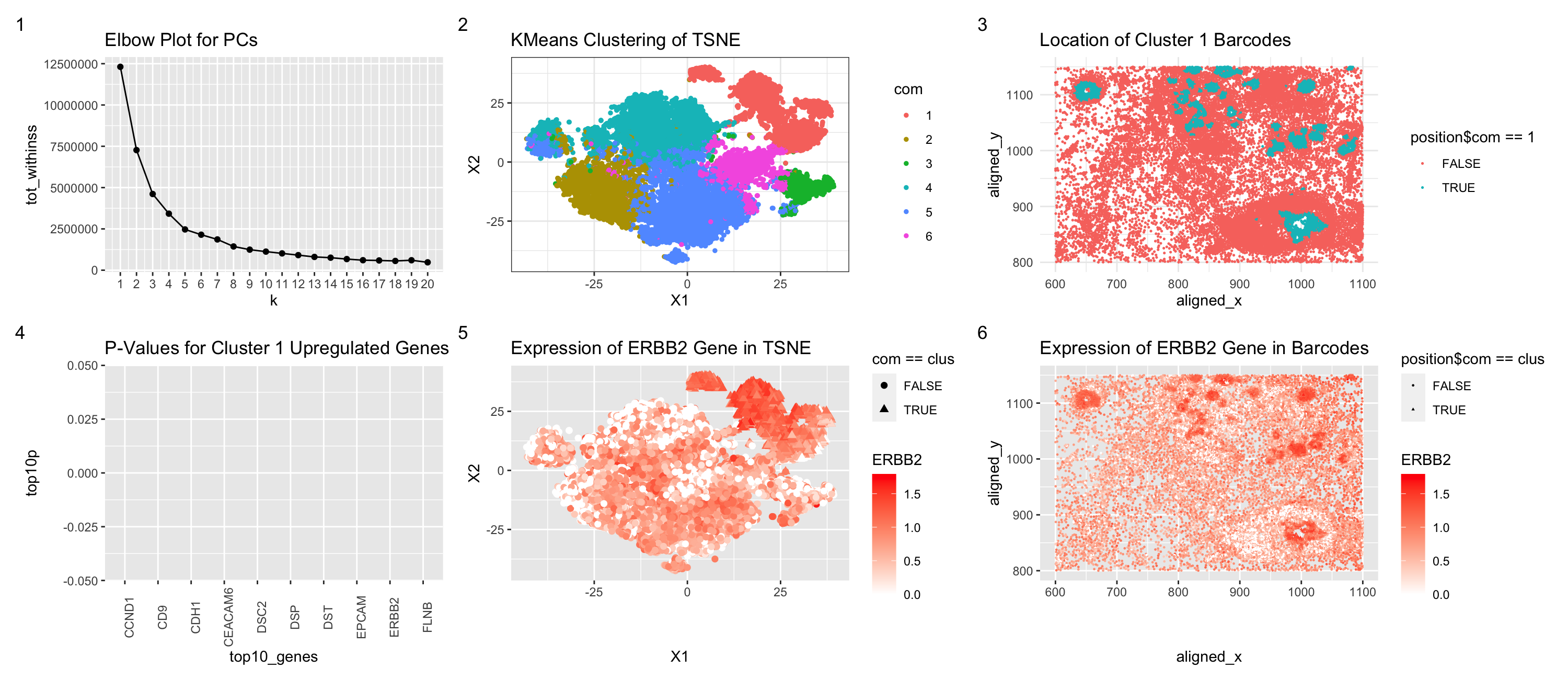
Figure Description
I switched from the Eevee dataset to the Pikachu dataset. As a result of the elbow plot, I judged that the optimal k for k-means clustering of the TSNE data was better at k = 6 rather than k = 4 for the Eevee dataset. This may be because there are more transcriptionally distinct cell-clusters in the cell-based Pikachu dataset. That may be because with the spot-based Eevee dataset, several cells may blend together as the resolution of the spot is larger than a cell. However, the cell-annotated data has a higher individual cell resolution. Furthermore, in order to find the cell type that was most similar to the one I found in the Eevee dataset, I performed calculations for each Pikachu cluster compared to the Eevee cluster using a two-sided t test to find the Pikachu cluster that was least different from the Eevee cluster. I then inserted the code from HW4 without much issue for creating the graphs, besides decreasing the spot size for the TSNE and physical location figures.
data <- read.csv('~/OneDrive/Documents/School/Johns Hopkins/Spring 2024/eevee.csv.gz', row.names=1)
data[1:5,1:5]
pos <- data[,2:3]
gexp <- data[, 4:ncol(data)]

topgene <- names(sort(apply(gexp, 2, var), decreasing=TRUE)[1:1000])
gexp <- gexpfilter <- gexp[,topgene]

gexpnorm <- log10(gexp/rowSums(gexp) * mean(rowSums(gexp))+1)

pcs <- prcomp(gexpnorm)

# tsne
library(Rtsne)
emb <- Rtsne(pcs$x[,1:20])$Y # faster than tSNE on genes

library(purrr)

tot_withinss <- map_dbl(1:10,  function(k){
  model <- kmeans(x = emb, centers = k)
  model$tot.withinss
})
# Generate a data frame containing both k and tot_withinss
elbow_df <- data.frame(
  k = 1:10,
  tot_withinss = tot_withinss
)

library(ggplot2)
# Plot the elbow plot -> chose k = 4 https://www.r-bloggers.com/2020/05/how-to-determine-the-number-of-clusters-for-k-means-in-r/
elbow <- ggplot(elbow_df, aes(x = k, y = tot_withinss)) +
  geom_line() + geom_point()+
  scale_x_continuous(breaks = 1:10)

com <- as.factor(kmeans(gexpnorm, centers=4)$cluster)

#plot tsne with clusters
p1 <- ggplot(data.frame(emb, com)) +
  geom_point(aes(x = X1, y = X2, col=com), size=1) +
  theme_bw()

#plot location of clusters
position <- data.frame(pos, com)

physical <- ggplot(position) +
  geom_point(aes(x = aligned_x,
                 y=aligned_y,
                 col= position$com == 4),
             size=1) +
  theme_minimal()

#finding differentially expressed genes
gexpnorm$cluster <- com

results <- sapply(colnames(gexp), function(g) {
  t.test(gexpnorm[com == 4, g],
         gexpnorm[com != 4, g],
         alternative = "greater")$p.val
})
results

# find p values https://r-graph-gallery.com/218-basic-barplots-with-ggplot2.html
top10p <- sort(results, decreasing = FALSE)[1:10]

top10p

top10genes <- rownames(data.frame(top10p))

genes <- data.frame(top10p, top10genes)

#https://guslipkin.medium.com/reordering-bar-and-column-charts-with-ggplot2-in-r-435fad1c643e
#plot p values of top 10 upregulated genes
top10_genes <- reorder(top10genes, top10p)

p_values <- ggplot(genes, aes(x= top10_genes, y = top10p)) + geom_bar(stat='identity')

c4genes <- data.frame(gexpnorm[com == 4,][, top10genes])

nonc4genes <- data.frame(gexpnorm[com != 4,][, top10genes])

#https://www.geeksforgeeks.org/how-to-find-mean-of-dataframe-column-in-r/
#cluster 4 gene expressions
avg <- sapply(1:10, function(g) {
  mean(c4genes[, g])
})

#non cluster 4 gene expressions
nonavg <- sapply(1:10, function(g) {
  mean(nonc4genes[, g])
})

# https://www.tutorialspoint.com/how-to-create-a-replicated-list-of-a-list-in-r#:~:text=The%20replication%20of%20list%20of,(x)%2C5).
# https://www.digitalocean.com/community/tutorials/r-melt-and-cast-function

df1 <- data.frame(Cluster_4 = avg, Cluster_1to3 = nonavg)

df1 <- as.data.frame(melt(df1))
df1_new <- data.frame(df1, rep(colnames(c4genes), 2))
colnames(df1_new) <- c("Cluster", "Expression", "Gene")

# plot to display upregulated genes
upreg_genes <- ggplot(df1_new, aes(x = Gene, y = Cluster, fill = Expression)) +
  geom_tile() + scale_fill_gradient(low="white", high="red")

#choose gene APOD
apod_tsne <- ggplot(data.frame(emb, com, gexpnorm['APOD'])) +
  geom_point(aes(x = X1, y = X2, col = APOD, shape = com == 4), size=2) +
  scale_color_gradient(low="white", high="red")

apod_physical <- ggplot(data.frame(position, gexpnorm['APOD'])) +
  geom_point(aes(x = aligned_x, y=aligned_y, col= APOD, shape = position$com == 4),
             size=2) + scale_color_gradient(low="white", high="red")

# https://patchwork.data-imaginist.com/articles/guides/annotation.html
library(patchwork)


# DATA FOR PIKACHU
data <- read.csv('~/OneDrive/Documents/School/Johns Hopkins/Spring 2024/pikachu.csv.gz', row.names=1)
#data parsing changed
data[1:5,1:5]
pos <- data[, 4:5]
gexp <- data[, 6:ncol(data)]
rownames(pos) <- rownames(gexp) <- data$cell_id
cell_area <- data$cell_area
names(cell_area) <- data$cell_id
head(cell_area)

gexpnorm_p <- log10(gexp/rowSums(gexp) * mean(rowSums(gexp))+1)

orig_columns <- colnames(gexpnorm_p)

pcs <- prcomp(gexpnorm_p)

# tsne
library(Rtsne)
emb <- Rtsne(pcs$x[,1:20])$Y # faster than tSNE on genes

library(purrr)

tot_withinss <- map_dbl(1:20,  function(k){
  model <- kmeans(x = emb, centers = k)
  model$tot.withinss
})
# increased number of k
# Generate a data frame containing both k and tot_withinss
elbow_df <- data.frame(
  k = 1:20,
  tot_withinss = tot_withinss
)

library(ggplot2)
# Plot the elbow plot -> changed and chose k = 20 https://www.r-bloggers.com/2020/05/how-to-determine-the-number-of-clusters-for-k-means-in-r/
elbow <- ggplot(elbow_df, aes(x = k, y = tot_withinss)) +
  geom_line() + geom_point()+
  scale_x_continuous(breaks = 1:20)

#chose k = 6

elbow

com <- as.factor(kmeans(gexpnorm_p, centers=6)$cluster)

#plot tsne with clusters
p1 <- ggplot(data.frame(emb, com)) +
  geom_point(aes(x = X1, y = X2, col=com), size=1) +
  theme_bw()

p1

#plot physical location of clusters
position <- data.frame(pos, com)

#I changed the size of points to represent cells
physical <- ggplot(position) +
  geom_point(aes(x = aligned_x,
                 y=aligned_y,
                 col= position$com == 1),
             size=.25) +
  theme_minimal()

physical

#finding differentially expressed genes
gexpnorm_p$cluster <- com

#find common genes
names <- intersect(colnames(gexpnorm_p), colnames(gexpnorm))

gexpnorm_p_names <- gexpnorm_p[,names]

gexpnorm_names <- gexpnorm[,names]

names <- names[1:(length(names)-1)]

# new p value loop
# evidently, cluster 1 of the pikachu data

results1 <- sapply(names, function(g) {
  t.test(gexpnorm_p_names[gexpnorm_p_names$cluster == 1, g],
         gexpnorm_names[gexpnorm_names$cluster == 4, g])$p.val
})

results2 <- sapply(names, function(g) {
  t.test(gexpnorm_p_names[gexpnorm_p_names$cluster == 2, g],
         gexpnorm_names[gexpnorm_names$cluster == 4, g])$p.val
})

results3 <- sapply(names, function(g) {
  t.test(gexpnorm_p_names[gexpnorm_p_names$cluster == 3, g],
         gexpnorm_names[gexpnorm_names$cluster == 4, g])$p.val
})

results4 <- sapply(names, function(g) {
  t.test(gexpnorm_p_names[gexpnorm_p_names$cluster == 4, g],
         gexpnorm_names[gexpnorm_names$cluster == 4, g])$p.val
})

results5 <- sapply(names, function(g) {
  t.test(gexpnorm_p_names[gexpnorm_p_names$cluster == 5, g],
         gexpnorm_names[gexpnorm_names$cluster == 4, g])$p.val
})

results6 <- sapply(names, function(g) {
  t.test(gexpnorm_p_names[gexpnorm_p_names$cluster == 6, g],
         gexpnorm_names[gexpnorm_names$cluster == 4, g])$p.val
})

results <- data.frame(results1 = results1, results2 = results2,
                      results3 = results3, results4 = results4,
                      results5 = results5, results6 = results6)

colMeans(results, na.rm = TRUE)

#RETURN TO CODE -> choose cluster with lowest p value

clus <- 1

results_p <- sapply(orig_columns, function(g) {
  t.test(gexpnorm_p[com == clus, g],
         gexpnorm_p[com != clus, g],
         alternative = "greater")$p.val
})
results_p

library(reshape2)

# find p values https://r-graph-gallery.com/218-basic-barplots-with-ggplot2.html
top10p <- sort(results_p, decreasing = FALSE)[1:10]

top10genes <- rownames(data.frame(top10p))

genes <- data.frame(top10p, top10genes)

#https://guslipkin.medium.com/reordering-bar-and-column-charts-with-ggplot2-in-r-435fad1c643e
#plot p values of top 10 upregulated genes
top10_genes <- reorder(top10genes, top10p)

p_values <- ggplot(genes, aes(x= top10_genes, y = top10p)) + geom_bar(stat='identity')

c4genes <- data.frame(gexpnorm_p[com == clus,][, top10genes])

nonc4genes <- data.frame(gexpnorm_p[com != clus,][, top10genes])

#https://www.geeksforgeeks.org/how-to-find-mean-of-dataframe-column-in-r/
#cluster of interest gene expressions
avg <- sapply(1:10, function(g) {
  mean(c4genes[, g])
})

#non cluster of interest gene expressions
nonavg <- sapply(1:10, function(g) {
  mean(nonc4genes[, g])
})

nonavg

# https://www.tutorialspoint.com/how-to-create-a-replicated-list-of-a-list-in-r#:~:text=The%20replication%20of%20list%20of,(x)%2C5).
# https://www.digitalocean.com/community/tutorials/r-melt-and-cast-function

df1 <- data.frame(Cluster_4 = avg, Cluster_1to3 = nonavg)

df1 <- as.data.frame(melt(df1))

df1_new <- data.frame(df1, rep(colnames(c4genes), 2))
df1_new

colnames(df1_new) <- c("Cluster", "Expression", "Gene")

# plot to display upregulated genes
upreg_genes <- ggplot(df1_new, aes(x = Gene, y = Cluster, fill = Expression)) +
  geom_tile() + scale_fill_gradient(low="white", high="red")

#choose gene of interest
com

gene <- "ERBB2"

rnase_tsne <- ggplot(data.frame(emb, com, gexpnorm_p['ERBB2'])) +
  geom_point(aes(x = X1, y = X2, col = ERBB2, shape = com == clus), size=2) +
  scale_color_gradient(low="white", high="red")

rnase_tsne

rnase_physical <- ggplot(data.frame(position, gexpnorm_p['ERBB2'])) +
  geom_point(aes(x = aligned_x, y=aligned_y, col= ERBB2, shape = position$com == clus),
             size=.5) + scale_color_gradient(low="white", high="red")

rnase_physical

# https://patchwork.data-imaginist.com/articles/guides/annotation.html
library(patchwork)

# https://www.datanovia.com/en/blog/ggplot-axis-ticks-set-and-rotate-text-labels/#:~:text=geom_boxplot()%20p-,Change%20axis%20tick%20mark%20labels,to%20rotate%20the%20tick%20text.
elbow <- elbow + ggtitle("Elbow Plot for PCs")
p1 <- p1 + ggtitle("KMeans Clustering of TSNE")
physical <- physical + ggtitle("Location of Cluster 1 Barcodes")
p_values <- p_values + ggtitle("P-Values for Cluster 1 Upregulated Genes") + theme(axis.text.x = element_text(angle = 90))
rnase_tsne <- rnase_tsne + ggtitle("Expression of ERBB2 Gene in TSNE")
rnase_physical <- rnase_physical + ggtitle("Expression of ERBB2 Gene in Barcodes")


elbow + p1 + physical + p_values + rnase_tsne + rnase_physical + plot_annotation(tag_levels = '1')