Pikachu dataset: Interpreting cell cluster through dimensionality reduction and differential gene expression analysis

Describe what you changed and why you think you had to change it.
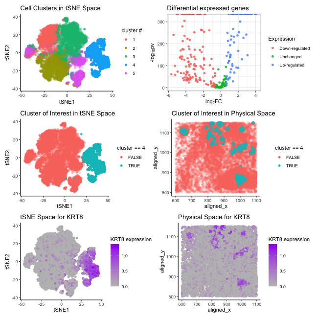
I switched from Eevee dataset to Pikachu dataset. In my previous visualization, I performed K means clustering with optimal K=3. I changed to K=5 this time after determining the optimal number of clusters to be 5 by plotting the percentage of variance explained against the number of clusters (elbow method). Additionally, I identified a “new” cluster of interest (#4) as a result of this change, however, I observed that the “new” cluster of interest shares the same spatial information as the previous cluster chosen (same aligned-x and aligned-y positions in the physical space). Previously, I hypothesized this particular cluster likely matches the profile with epithelial cells. Hence, picking this “new” cluster (#4) might help me to interpret the same cell cluster based on the consistency of the spatial information in the physical space.
I also changed my interested gene from ELF3 to KRT8. After performing a differential gene expression analysis and generating a volcano plot, I found three interested genes that are up-regulated(KRT8, ELF3, and CDH1). Nevertheless, KRT8 is most expressed in cluster 4, providing more relevant information visually.
Describe why you found the same cell type as the one in your previous visualization
As I mentioned, I found KRT8 and ELF3 are both up-regulated in cluster 4 through differential gene expression analysis and previously speculated about this cluster to match the profile with epithelial cells. Although KRT8 is identified as a pan-cancer early biomarker and is associated with many cell types[1], it is preferentially expressed in many simple epithelial cells, such as hepatocytes, pancreatic acinar and islet cells, and proximal tubular kidney epithelial cells [2]. Additionally, KRT8 is found upregulated in clear cell renal cell carcinoma , gastric cancer, breast cancer, and lung cancer. Aberrantly high expression of KRT8 has been found to be associated with multiple tumor progressions including cell migration[3]. This finding matches other evidence suggesting KRT8 being one of the key genes related to epithelial-mesenchymal transition (EMT) as epithelial cells undergoing EMT exhibit enhanced migratory capacity.
Following this clue above, another interesting finding is that all three identified up-regulated genes (KRT8, ELF3, and CDH1) are highly correlated because they all play crucial roles in EMT/MET pathway in LUAD (Lung adenocarcinoma)[4]. This might point out more directions to further investigate the relationship between this specific cell cluster and its potential biomarkers.
Reference:
-
Scott, M. K. D., Limaye, M., Schaffert, S., West, R., Ozawa, M. G., Chu, P., Nair, V. S., Koong, A. C., & Khatri, P. (2021). A multi-scale integrated analysis identifies KRT8 as a pan-cancer early biomarker. Pacific Symposium on Biocomputing. Pacific Symposium on Biocomputing, 26, 297–308.
-
Tan H., Jiang W., He Y., Wang D., Wu Z., Wu D., Gao L., Bao Y., Shi J., Liu B., Ma L., Wang L. KRT8 upregulation promotes tumor metastasis and is predictive of a poor prognosis in clear cell renal cell carcinoma. Oncotarget. 2017; 8: 76189-76203. Retrieved from https://www.oncotarget.com/article/19198/text/
-
Chen H, Chen X, Pan B, Zheng C, Hong L and Han W (2022) KRT8 Serves as a Novel Biomarker for LUAD and Promotes Metastasis and EMT via NF-κB Signaling. Front. Oncol. 12:875146. doi: 10.3389/fonc.2022.875146
-
Wang, W., He, J., Lu, H., Kong, Q., & Lin, S. (2020). KRT8 and KRT19, associated with EMT, are hypomethylated and overexpressed in lung adenocarcinoma and link to unfavorable prognosis. Bioscience reports, 40(7), BSR20193468. https://doi.org/10.1042/BSR20193468
library(ggplot2)
library(Rtsne)
library(tidyverse)
library(RColorBrewer)
library(patchwork)

data <- read.csv("pikachu.csv.gz", row.names = 1)
pos = data[,4:5]
gexp = data[,6:ncol(data)]

# normalize data
gexp <-gexp[,colSums(gexp)>1000]
totalgen_exp <- rowSums(gexp)
norm_gexp <- gexp/totalgen_exp * median(totalgen_exp)
norm_gexp <- log10(norm_gexp + 1)

set.seed(200)
# PCA
pcs <- prcomp(norm_gexp)
# tSNE on 20 pcs
tsne_genes_res <- Rtsne(pcs$x[,1:20], dims = 2, perplexity = 30)

# pick optimal k using elbow method
# ref: https://www.r-bloggers.com/2017/02/finding-optimal-number-of-clusters/
k.max <- 8
wss <- sapply(1:k.max,
              function(k){kmeans(norm_gexp, k, nstart=50,iter.max = 15 )$tot.withinss})
# elbow plot
plot(1:k.max, wss,
     type="b", pch = 19, frame = FALSE,
     xlab="Number of clusters K",
     ylab="Total within-clusters sum of squares")

# pick k=5
com <- as.factor(kmeans(norm_gexp, center=5)$cluster)
data <- data.frame(pos, tsne_genes_res$Y, cellType = com)

alpha <- ifelse(data$cellType ==4, 0.85, 0.2)
# Reduced dimensional space visualization of all 5 clusters
p <- ggplot(data) +
  geom_point(aes(x = X1, y = X2, col=cellType), alpha = alpha) +
  labs(title = 'Cell Clusters in tSNE Space',
       x = 'tSNE1', y = 'tSNE2', col = "cluster #") +
  theme_bw() +
  theme_classic()

# Panel 1: Reduced dimensional space visualization of the cluster
p1 <- ggplot(data) +
  geom_point(aes(x = X1, y = X2, color = (cellType ==4)), alpha = alpha) +
  theme_bw() +
  labs(title = "Cluster of Interest in tSNE Space",
       x = "tSNE1", y = "tSNE2", col = "cluster == 4") +
  theme_classic()


# Panel 2: Physical space visualization of the cluster
p2 <- ggplot(data) +
  geom_point(aes(x = aligned_x, y = aligned_y, color = (cellType ==4)), alpha = alpha) +
  theme_bw() +
  labs(title = "Cluster of Interest in Physical Space",
       col = "cluster == 4") +
  theme_classic()


# differential expression analysis
#p-value
pv <- sapply(colnames(norm_gexp), function(i){
  wilcox.test(group1 <- norm_gexp[com == 4, i], norm_gexp[com != 4,i])$p.val
})

# Adjust p-values using the Benjamini-Hochberg correction
pv <- p.adjust(pv, method = "BH")

# log2 fold change
logfc <- sapply(colnames(norm_gexp), function(i){
  log2(mean(norm_gexp[com == 4, i])/mean(norm_gexp[com != 4, i]))
})


# Panel 3: volcano plot for differentially expressed genes
# ref: https://samdsblog.netlify.app/post/visualizing-volcano-plots-in-r/
volc_df <- data.frame(pv, logfc)
volc_df <- volc_df %>%
  mutate(
    Expression = case_when(logfc >= 0.6 & pv <= 0.05 ~ "Up-regulated",
                           logfc <= -0.6 & pv <= 0.05 ~ "Down-regulated",
                           TRUE ~ "Unchanged")
  )

p3 <- ggplot(volc_df , aes(logfc, -log(pv,10))) +
  geom_point(aes(color = Expression), alpha = 0.85) +
  ylim(-.05, 320) +
  xlab(expression("log"[2]*"FC")) +
  ylab(expression("-log"[10]*"pv")) +
  ggtitle("Differential expressed genes")+
  theme_bw()
  theme_minimal() +
  guides(colour = guide_legend(override.aes = list(size=1.5)))

# Differentially expressed gene: krt8
deg_df <- cbind(data, krt8 = norm_gexp$KRT8)
# Panel 4: Visualization of one DEG in reduced dimensional space
p4 <- ggplot(deg_df) +
  geom_point(aes(x = X1, y = X2, color= krt8)) +
  scale_color_gradient(low="grey", high="purple")+
  labs(title = "tSNE Space for KRT8",
       x = "tSNE1", y = "tSNE2", col = "KRT8 expression") +
  theme_classic()

# Panel 5: Visualization of one DEG in physical space
p5 <- ggplot(deg_df) +
  geom_point(aes(x = aligned_x, y = aligned_y, color= krt8)) +
  scale_color_gradient(low="grey", high="purple")+
  labs(title = "Physical Space for KRT8", col = "KRT8 expression") +
  theme_classic()

png(file="hw5_plot.png",
    width=650, height=650)
(p | p3)/ (p1 | p2) / (p4 | p5)
dev.off()