Cell Cluster Identification and Validation in Breast Tumor Tissue

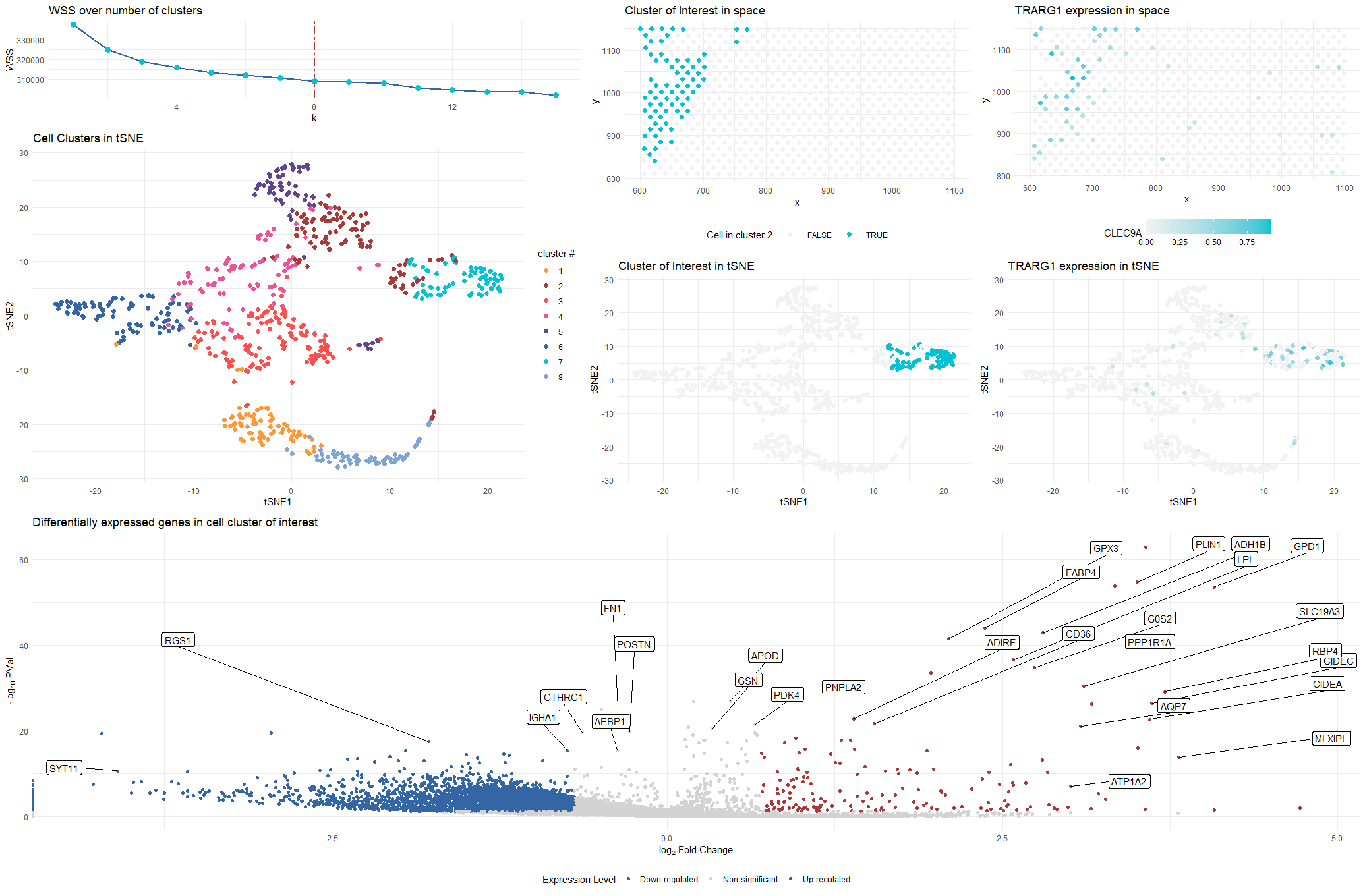
### Plot Description This visualization presents differential gene expression to validate cell type identification by k-means on 2D tSNE space.

• The spatial-transcriptomics data on breast tumor tissue is preprocessed by removing cells with total gene counts below 0.2* average of total gene counts, normalized by total gene counts, and log-scaled.

• The 8 cell clusters (see WSS curve for choice of k) are encoded by different colors in tSNE space to show the performance of k-means clustering.

• A cluster is selected as cluster of interest by TARG1 count and identified in both tSNE and physical space with the same color used in the 8-cluster plot.

• The most differentially expressed genes are computed in the selected cluster through two-sided Wilcox test, and demonstrated on the volcano plot.

• The chracteristic TRARG1 gene’s distribution is plotted in both tSNE and physical space

  Changes made

1. Adapt to the columns of eevee dataset
2. Change the number of PCs and Clusters based of scree plot and WSS
3. Deal with NaN value in pvs
4. attempt to use a more unique marker for human dendritic cells, so change the target cluster to Adipocytes (TRARG1)
5. change the color as directed by TA feedback from HW4

ref: https://www.proteinatlas.org/ENSG00000184811-TRARG1

Source Code

## load dataset
data <- read.csv('C:/Users/ivych/OneDrive - Johns Hopkins/Classes/Data Visualization/eevee.csv.gz', row.names = 1)
data[1:5,1:5]

# install.packages("Rtsne")
## import libraries
library(ggplot2)
library(gridExtra)
library(Rtsne)

## set theme
#ref: https://www.color-hex.com/color-palette/1022322
xiao_plt <- c(     
              "#FF983B",
              "#AA3A39",
              "#FE4E4E",
              "#EE5397", 
              "#634490",
              "#3466A5",
              "#00C4D4",
              "#7fa4d6")

## data selection
pos <- data[, 2:3]
gexp <- data[, 4:ncol(data)]
gexp_mean <- mean(rowSums(gexp))
good.cells <-rownames(gexp)[rowSums(gexp) > 0.2*gexp_mean]
nrow(pos[good.cells,])
nrow(pos)
pos <- pos[good.cells,]
gexp <- gexp[good.cells,]

## normalization
gexp_norm <- gexp*median(rowSums(gexp))/rowSums(gexp)
gexp_log <- log10(gexp_norm+1)
mat <- unique(gexp_log)

#scree plot for pcs
x <- 1:15
pcs <- prcomp(mat)

par(mfrow=c(1,1))
data_scree <- data.frame(x = x, std = pcs$sdev[1:15])

ggplot(data_scree, aes(x, std)) +
  geom_line(color = xiao_plt[4], size = 1) +
  geom_point(color = xiao_plt[3], size = 3) +
  labs(title = "Scree plot", x = "Number of PCs", y = "STD") +
  theme_minimal()
#pcs = 4

#pcs and tsne
pcs_result <- pcs$x[,1:4]
tsne_result <- Rtsne::Rtsne(pcs_result)

## elbow method for clustering
wss <- numeric(15)
for (i in 1:15) {
  wss[i] <- sum(kmeans(mat, centers = i)$withinss)
}

data_elbow <- data.frame(x = x, wss = wss)
p_elbow <- ggplot(data_elbow, aes(x, wss)) +
  geom_segment(col = xiao_plt[2], size=1, linetype = 'twodash',
               aes(x = 8, y = Inf, xend = 8, yend = -Inf)) + 
  geom_line(color = xiao_plt[6], size = 1) +
  geom_point(color = xiao_plt[7], size = 3) +
  labs(title = "WSS over number of clusters", x = "k", y = "WSS") +
  theme_minimal()
p_elbow

## K-means
#k = 8 seems to give the optimal result
com = kmeans(mat, center  = 8)
df <- data.frame(pos, tsne_result$Y, celltype=as.factor(com$cluster))
head(df)
p_k <- ggplot(df) + 
  geom_point(size = 2,aes(x = X1, y = X2, col=celltype)) +
  labs(title = 'Cell Clusters in tSNE',
       x = 'tSNE1', y = 'tSNE2', col = "cluster #") +
  theme_minimal() + # theme(legend.position = "none") + 
  scale_colour_manual(values = xiao_plt)
p_k

# pick cluster of interest
coi <- 7

#cluster of interest in the tsne space
p_c1 <- ggplot(df) + 
  geom_point(size = 2,aes(x = X1, y = X2, col=(celltype==coi))) + 
  labs(title = 'Cluster of Interest in tSNE',
       x = 'tSNE1', y = 'tSNE2',col="in cluster 2") +
  theme_minimal() + theme(legend.position = "none") + 
  scale_colour_manual(values = c("grey95",xiao_plt[coi]))
p_c1

#cluster of interest in the physical space
p_c2 <- ggplot(df) + 
  geom_point(size = 2, aes(x = aligned_x, y = aligned_y, col=(celltype==coi))) + 
  labs(title = 'Cluster of Interest in space',
       x = 'x', y = 'y',col="Cell in cluster 2") +
  theme_minimal() + theme(legend.position = "bottom", legend.key.size = unit(1, "cm")) + 
  scale_colour_manual(values = c("grey95",xiao_plt[coi]))
p_c2


## Double-sided wilcox test to identify differential expression
cluster.oi<- names(which(com$cluster == coi))
cluster.ot <- names(which(com$cluster != coi))

#differential genes
genes <- colnames(mat)
pvs <- sapply(genes, function(g) {
  oi <- mat[cluster.oi, g]
  ot <- mat[cluster.ot, g]
  wilcox.test(oi, ot, alternative="two.sided")$p.val})
pvs[is.na(pvs)] = 0.06

names(which(pvs < 1e-8))
head(sort(pvs), n=20)

#fold change
log2fc <- sapply(genes, function(g) {
  oi <- mat[cluster.oi, g]
  ot <- mat[cluster.ot, g]
  log2(mean(oi)/mean(ot))})
log2fc[is.na(log2fc)] = 0

#volcano plot
df_volcano <- data.frame(pvs, log2fc)
exp_sig <- apply(df_volcano, 1, function(g) {
  if (g[2] >= log(2) & g[1] <= 0.05) {out = "Up-regulated"} 
  else if (g[2] <= -log(2) & g[1] <= 0.05) {out = "Down-regulated"} 
  # else if (g[2] == 0 & g[1] == 0.06) {out = "NaN"} 
  else {out = "Non-significant"}
  out})
data_deg <- cbind(df_volcano, exp_sig)

#install.packages("ggrepel")


p_volc <- ggplot(data_deg, aes(y=-log10(pvs), x=log2fc)) + 
  scale_color_manual(values = c(xiao_plt[6], "lightgray", xiao_plt[2])) +
  geom_point(aes(col = exp_sig)) +
  ggrepel::geom_label_repel(label=rownames(data_deg)) +
  xlab(expression("log"[2]*" Fold Change")) + 
  ylab(expression("-log"[10]*" PVal")) +
  theme_minimal()+
  theme(legend.position = 'bottom') +
  labs(title = 'Differentially expressed genes in cell cluster of interest',
       col = "Expression Level")
p_volc

# Visualize CD1C
# https://bmccancer.biomedcentral.com/articles/10.1186/s12885-023-10558-2#:~:text=CD1C%20is%20an%20important%20part%20of%20the%20TME,and%20a%20new%20treatment%20target%20for%20breast%20cancer.

df_clec9a <- cbind(df,CLEC9A = mat$TRARG1)

p_clec9a <-ggplot(df_clec9a) + 
  geom_point(size = 2,aes(x = aligned_x, y = aligned_y, col = CLEC9A)) +
  theme_minimal() + theme(legend.position="bottom", legend.key.width = unit(1, "cm")) +
  labs(title = 'TRARG1 expression in space',
       x = 'x', y = 'y') +
  scale_color_gradient(low = 'grey95', high=xiao_plt[coi]) 
p_clec9a

p_clec9a2 <- ggplot(df_clec9a) + 
  geom_point(size = 2,aes(x = X1, y = X2, col = CLEC9A)) +
  theme_minimal()+ theme(legend.position="none", legend.key.size = unit(0.2, "cm")) +
  labs(title = 'TRARG1 expression in tSNE',
       x = 'tSNE1', y = 'tSNE2') +
  scale_color_gradient(low = 'grey95', high=xiao_plt[coi]) 
p_clec9a2

#plot panel arrangement
layout <- rbind(c(1,1,1,3,3,4,4),
                c(2,2,2,3,3,4,4),
                c(2,2,2,5,5,6,6),
                c(2,2,2,5,5,6,6),
                c(7,7,7,7,7,7,7),
                c(7,7,7,7,7,7,7),
                c(7,7,7,7,7,7,7))
grid.arrange(p_elbow,p_k,
             p_c2,p_clec9a,
             p_c1,p_clec9a2,
             p_volc,
             layout_matrix = layout)