Exploring cell type using differential gene expression through KMeans clustering

Write a description of what you changed and why you think you had to change it.
I switched from the Eevee to the Pikachu dataset. I previously performed KMeans clustering with k=3. Now I performed k-means clustering with k=10. This is because I found the optimal K based on total withinness to be 10 for this dataset. I think there are more optimal number of transcriptionally distinct cell-clusters in the single-cell resolution Pikachu dataset as compared to the spot-based Eevee dataset because single-cell resolution data allows for more granular analysis of gene expression within individual cells. This higher resolution enables the detection of subtle transcriptional differences between cells.
After finding optimal K, I applied KMeans clustering on the normalized gene expression data. Because of the absence of differential expression of ‘DSP’ in all 10 clusters, I decided to pick one cluster characterized by scattered spatial distribution and identified the upregulated gene in that cluster and repeated the same previous analysis. I chose a cluster which was scattered spatially (turquoise in color). I was interested to see which gene is upregulated in this cluster. I performed t-test to see the upregulated genes in this cluster of interest, and found that KRT7 (pvalue 1.5182e-99) was the top gene that was upregulated, unlike ‘DSP’ in my previous analysis for spot-based dataset. Further, I visualized KRT7 in the physical space and in PCA space.
Create a multi-panel data visualization and write a description to convince me you found the same cell-type.
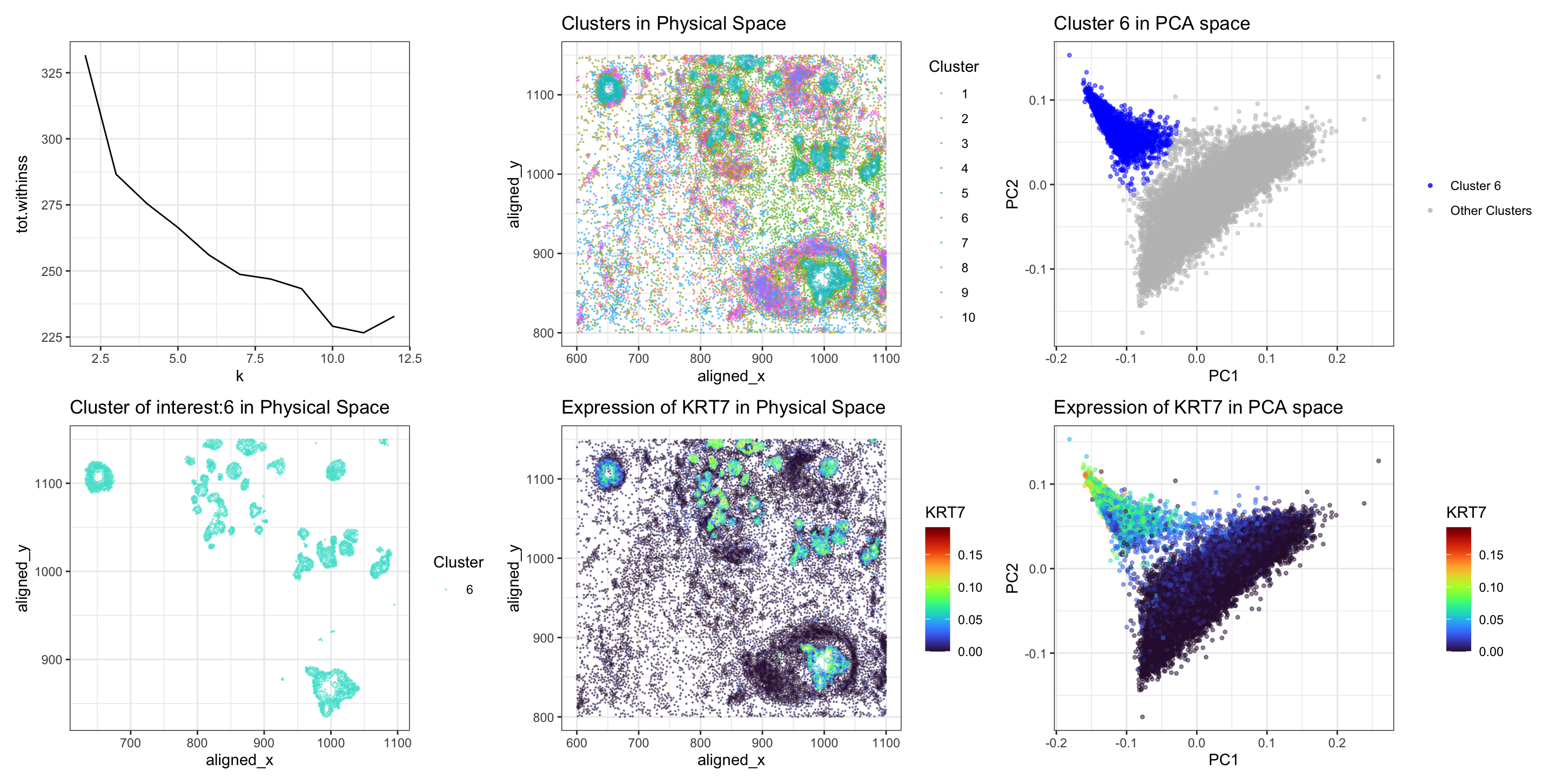
Upon transitioning from the Eevee to the Pikachu single-cell resolution dataset. Initially, total withiness was used find optimal k (panel 1). Subsequently, I visualized the clusters in physical space (panel 2). A cluster exhibiting scattered spatial distribution (turquoise in color) was selected for further investigation, aiming to identify genes differentially upregulated (panel 4). I also visualized this cluster of interest (6) in comparison to others in the PCA space (panel 3). Cells in cluster 6 are clustered together on PC axis in blue color.
Conducting a Wilcox-test revealed ‘KRT7’ as the top upregulated gene within the selected cluster, exhibiting a highly significant p-value (pvalue 1.5182e-99). This finding was different from the previous analysis, which identified DSP as the predominant upregulated gene, underscoring the nuanced transcriptional heterogeneity inherent in single-cell resolution datasets.
Then, I visualized the spatial landscape of KRT7 expression within the tissue. In physical space (panel 5), cells within the selected cluster exhibited intense KRT7 expression, depicted by vibrant turquoise-yellow coloring. Similarly, PCA-based visualization (panel 6) reaffirmed the clustering of cells (turquoise-yellow) with elevated KRT7 expression corresponding to the location of cluster 6 in PCs, suggesting a distinct transcriptional profile associated with this cell-type.
Integration of the above information with the known literature indicates that the identified cluster likely consists of epithelial cells characterized by high expression of the KRT7 gene. The known biology of KRT7, predominantly associated with epithelial cells in breast (glandular cells), and other tissues, offers a compelling framework for interpreting the observed expression pattern [1][2]. While the marker gene may differ from my previous analyses, the identification of epithelial cells remains consistent with my previous analysis.
[1] “NCBI Gene: KRT7 keratin 7 [Homo sapiens (human)] - Gene - NCBI.” National Center for Biotechnology Information, U.S. National Library of Medicine, www.ncbi.nlm.nih.gov/gene/3855.
[2] “The Human Protein Atlas: KRT7.” The Human Protein Atlas, www.proteinatlas.org/ENSG00000135480-KRT7/tissue.
library(viridis)
library(patchwork)
library(ggplot2)
data <- read.csv('/Users/nidhisoley/Desktop/GDataViz/pikachu.csv.gz', row.names=1)
# Drop first 5 columns for gene expression (cell_id, cell_area etc)
gexp <- data[, -c(1:5)]
rownames(gexp) <- data$cell_id
pos <- data[, 4:5]
gexpnorm <- gexp/rowSums(gexp)
pcs <- prcomp(gexpnorm)
#total withinness change with k
withinnes.list <-sapply(c(2:12), function(x) {
  print(x)
  tmp = kmeans(gexpnorm, centers = x)
  return(tmp$tot.withinss)} )
p0 <- ggplot(data.frame(k = c(2:12), tot.withinss = withinnes.list),
            aes(k, tot.withinss)) +
  geom_line()+theme_bw()
p0
#KMeans
clusters <- as.factor(kmeans(gexpnorm, centers = 10)$cluster)
p1 <- ggplot(data.frame(data, Cluster = clusters)) +
  geom_point(aes(x = aligned_x, y = aligned_y, col = Cluster), size=0.1, alpha=0.5) +
  theme_bw() +
  labs(title = "Clusters in Physical Space")
p1
#cluster of interest
cluster_of_interest <- 6
df <- data.frame(data, kmeans=(clusters))
df1 <- df[df$kmeans == cluster_of_interest,]
p2 <-ggplot(df1) + geom_point(aes(x = aligned_x, y=aligned_y, col=kmeans),
                              size=0.1,alpha=0.5) + theme_bw() +
  labs(title='Cluster of interest:6 in Physical Space')+
  labs(color='Cluster')+
  scale_color_manual(values = "turquoise")
p2
#pca
pca_df <- data.frame(PC1 = pcs$x[, 1], PC2 = pcs$x[, 2], Cluster = clusters)
cluster_1_df <- pca_df[pca_df$Cluster == cluster_of_interest, ]
p3 <- ggplot(pca_df, aes(x = PC1, y = PC2)) +
  geom_point(data = cluster_1_df, aes(col = "Cluster 6"), size = 0.9, alpha=0.5) +
  geom_point(data = pca_df[pca_df$Cluster != cluster_of_interest, ], aes(col = "Other Clusters"), size = 0.9, alpha=0.5) +
  scale_color_manual(values = c("Cluster 6" = "blue", "Other Clusters" = "gray")) +
  theme_bw() +
  labs(title = "Cluster 6 in PCA space",
       color = "Cluster") +
  guides(color = guide_legend(title = NULL))
p3
#t-test
results <- sapply(colnames(gexpnorm), function(g) {
  t.test(gexpnorm[clusters == cluster_of_interest, g],
         gexpnorm[clusters != cluster_of_interest, g],
         alternative = 'greater')$p.val
})
significant_genes <- names((sort(results,decreasing = FALSE)[1:50]))
significant_genes_df <- data.frame(Gene = significant_genes, p_value = results[significant_genes])
#KRT7
gene_of_interest <- 'KRT7'
p4 <- ggplot(data.frame(pos, gene = gexpnorm[, gene_of_interest])) +
  geom_point(aes(x = aligned_x, y = aligned_y, col = gene),  size=.1,alpha=0.5) +
  scale_color_viridis(option = 'H')+
  theme_bw() +
  labs(title = paste("Expression of", gene_of_interest, "in Physical Space"))+
  labs(color=gene_of_interest)
p5 <- ggplot(data.frame(pcs$x, gene = gexpnorm[, gene_of_interest])) +
  geom_point(aes(x = PC1, y = PC2, col = gene),  size=.9,alpha=0.5) +
  scale_color_viridis(option = 'H')+
  theme_bw() +
  labs(title = paste("Expression of", gene_of_interest, "in PCA space"))+
  labs(color=gene_of_interest)
p0+p1 +p3+p2+p4+p5
plot_layout(ncol = 3)