Identification of Epithelial Cell Cluster in Breast Cancer Tissue of Pikachu Data Set

Description of Visualization Changes
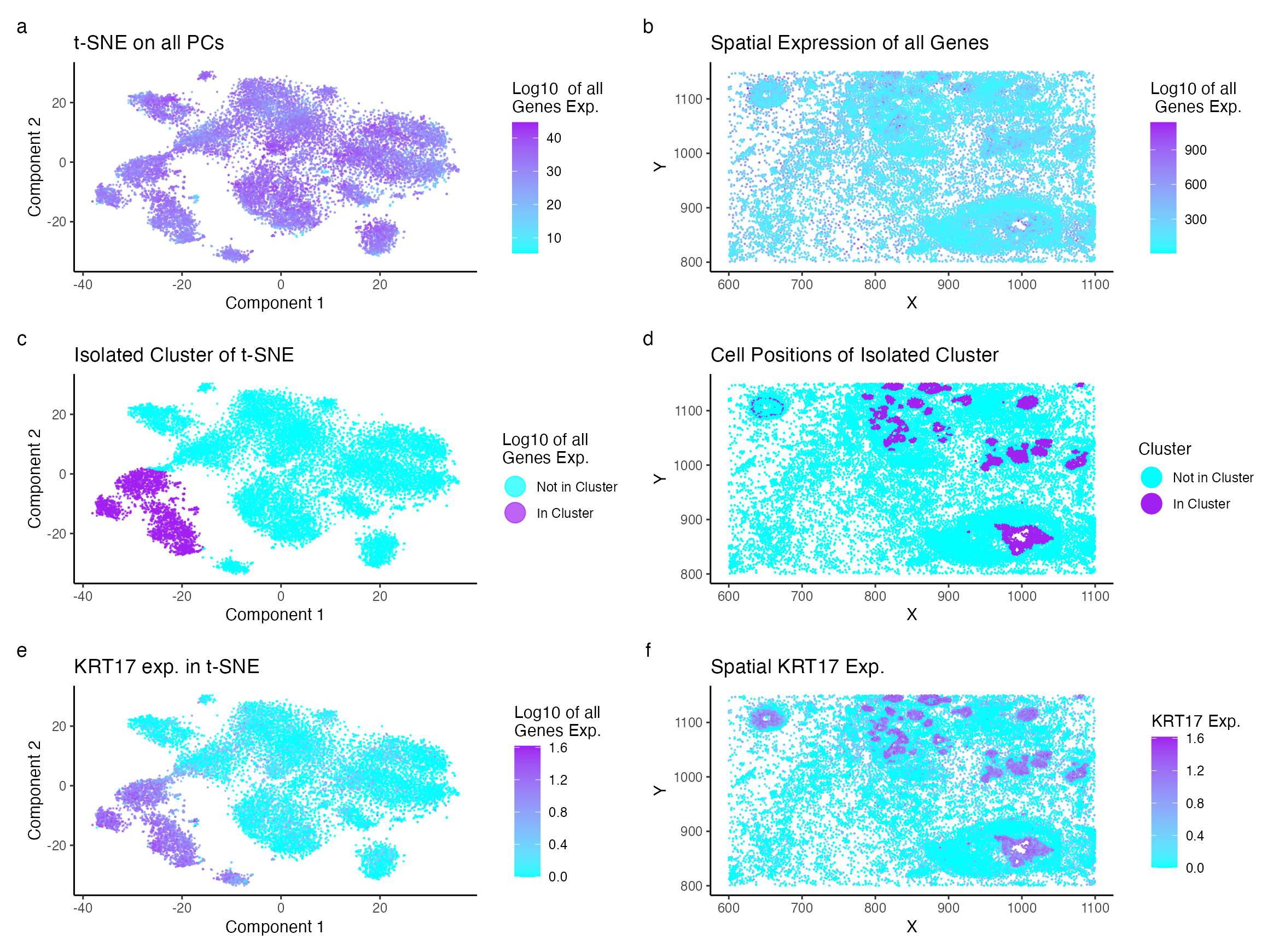
When visualizing the Eevee data set, I had visual analysis to determine the optimal number of clusters to be K=10. In the pikachu data set, I had initally used the elbow method to determine the optimal number of cluster to be K=8. However, visual analysis of gene expresion within the clusters lead to the conclusion the sample was over clustered as many genes identified in some clusters were also expressed in others. Thus, the clustering was changed to K=7. Additionally, the Pikachu data set, despite having a higher spatial resolution compared to the Eevee data set’s spot based technique, contains less genes (~300 vs ~18000 in Pikachu vs Eevee). As a result, the previously analyzed gene KRT80 was not present in the data set to confirm identification. ERBB2, KRT7, TACSTD2, CCND1, SERPINA3, KRT8, CEACAM6, MYLK, TCIM, and EPCAM were the most expressed genes in the isolated cluster. ERBB2 was not chosen for visualization due to its high expressivity in other clusters. Instead, KRT17, the second most unique gene, was chosen for further analysis.
Cell Type Interpretation:
KRT17 is a known epithial cell bio marker (Wang et al.). The gene encodes Keratin, and when unregulated, Depainto et al. concludes, is responsible for the proliferation of epithelial cells and tumor growth. Specifically for breast cancer, KRT17 functions as a promoter (Li et al.).
Wang et al.: https://www.ncbi.nlm.nih.gov/pmc/articles/PMC6689799/ Depainto et al.: https://www.ncbi.nlm.nih.gov/pmc/articles/PMC2947596/ Li et al.: https://www.dovepress.com/krt17-functions-as-a-tumor-promoter-and-regulates-proliferation-migrat-peer-reviewed-fulltext-article-CMAR
library(Rtsne)
library(ggplot2)
library(patchwork)
library(viridis)
set.seed(0)
data <- read.csv("/Users/knm/github/genomic-data-visualization-2024/data/pikachu.csv.gz", row.names = 1)

gexp <- data[, 6:ncol(data)]
topgene <- names(sort(apply(gexp, 2, var), decreasing=TRUE)[1:200])
gexp <- gexp[,topgene]

pos <- data[, 4:5]

gexpnorm <- log10(gexp/rowSums(gexp) * mean(rowSums(gexp))+1)
dim(gexp)

pcs <- prcomp(gexpnorm)
emb <- Rtsne(pcs$x)$Y

calculate_wss <- function(data, k_max) {
  wss <- numeric(k_max)

  for (k in 1:k_max) {
    kmeans_result <- kmeans(data, centers = k, nstart = 10)
    wss[k] <- kmeans_result$tot.withinss
  }

  return(wss)
}
k_max <- 10
wss <- calculate_wss(emb, k_max)
elbow_point <- which(diff(diff(wss)) == min(diff(diff(wss))))
plot(1:k_max, wss, type = "b", pch = 19, frame = FALSE,
     xlab = "Number of clusters", ylab = "Total within-cluster sum of squares")

com <- as.factor(kmeans(emb, centers=7)$cluster)

df <- data.frame(emb_1 = emb[,1], emb_2 = emb[,2],
                 com = com)

p1 <- ggplot(df) +
  geom_point(aes(x = emb_1, y = emb_2, color = com == 4), alpha = 0.7, size = 0.1) +
  scale_color_manual(values = c("TRUE" = "purple", "FALSE" = "cyan"),
                     labels = c("Not in Cluster", "In Cluster")) +
  guides(color = guide_legend(override.aes = list(size = 6))) +
  theme_classic() +
  labs(title = "Isolated Cluster of t-SNE", color = "Log10 of all \nGenes Exp.",
       x = "Component 1", y = "Component 2")
p1

p2 <- ggplot(df) +
  geom_point(aes(x = emb_1, y = emb_2, color = rowSums(gexpnorm)), alpha = 0.7, size = 0.1) +
  scale_color_gradient(low = "cyan", high = "purple") +
  theme_classic() +
  labs(title = "t-SNE on all PCs", color = "Log10  of all \nGenes Exp.",
       x = "Component 1", y = "Component 2")
p2


pv <- sapply(colnames(gexpnorm), function(i) {
  wilcox.test(gexpnorm[com == 4, i], gexpnorm[com != 4, i], alternative = "two.sided")$p.val
})
logfc <- sapply(colnames(gexpnorm), function(i) {
  log2(mean(gexpnorm[com == 4, i])/mean(gexpnorm[com != 4, i]))
})

plot_df <- data.frame(logfc = logfc, pv = -log10(pv))

p3 <- ggplot(plot_df, aes(x = logfc, y = pv)) +
  geom_point() +
  theme_classic() +
  labs(title = "logFC vs PV",
       x = "Log Fold Change",
       y = "-log10(p-value)")
p3


df_spatial <- data.frame(x = data$aligned_x, y = data$aligned_y, cluster = com)
p4 <- ggplot(df_spatial) +
  geom_point(aes(x = x, y = y, color = com == 4), size = 0.1) +
  scale_color_manual(values = c("TRUE" = "purple", "FALSE" = "cyan"),
                     labels = c("Not in Cluster", "In Cluster")) +
  guides(color = guide_legend(override.aes = list(size = 6))) +
  theme_classic() +
  labs(title = "Cell Positions of Isolated Cluster", color = "Cluster",
       x = "X", y= "Y")
p4


product <- -log10(pv) * logfc
top_genes <- names(sort(product, decreasing = TRUE))
print(top_genes)
gene_analysis <- top_genes[2]
top_genes[1:10]
p5 <- ggplot(df) +
  geom_point(aes(x = emb_1, y = emb_2, color = gexpnorm[,gene_analysis]), alpha = 0.7, size = 0.1) +
  scale_color_gradient(low = "cyan", high = "purple") +
  theme_classic() +
  labs(title = "KRT17 exp. in t-SNE", color = "Log10 of all \nGenes Exp.",
       x = "Component 1", y = "Component 2")
p5

df_spatial_2 <- data.frame(x = data$aligned_x, y = data$aligned_y, gene = gexpnorm[, gene_analysis])
p6 <- ggplot(df_spatial_2) +
  geom_point(aes(x = x, y = y, color = gene), size = 0.1) +
  scale_color_gradient(low = "cyan", high = "purple") +
  theme_classic() +
  labs(title = "Spatial KRT17 Exp.", color = "KRT17 Exp.",
       x = "X", y= "Y")
p6

df_spatial_3 <- data.frame(x = data$aligned_x, y = data$aligned_y, gene = rowSums(gexp))
p7 <- ggplot(df_spatial_3) +
  geom_point(aes(x = x, y = y, color = gene), size = 0.1) +
  scale_color_gradient(low = "cyan", high = "purple") +
  theme_classic() +
  labs(title = "Spatial Expression of all Genes", color = "Log10 of all \n Genes Exp.",
       x = "X", y= "Y")
p7

combined_plot <- p2 + p7 + p1 + p4 + p5 + p6 + plot_annotation(tag_levels = 'a') +
  plot_layout(ncol = 2) #p3
combined_plot
ggsave("/Users/knm/Library/CloudStorage/OneDrive-JohnsHopkins/Johns Hopkins [2021-2025]/Junior [2023-2024]/Genomics Data Visualization/Homework/hw5_kmukund1.png", combined_plot, width = 16.70*.7, height = 12.44*.7, units = "in", dpi = 200)