Analyzing for Breast Glandular Cells: V2

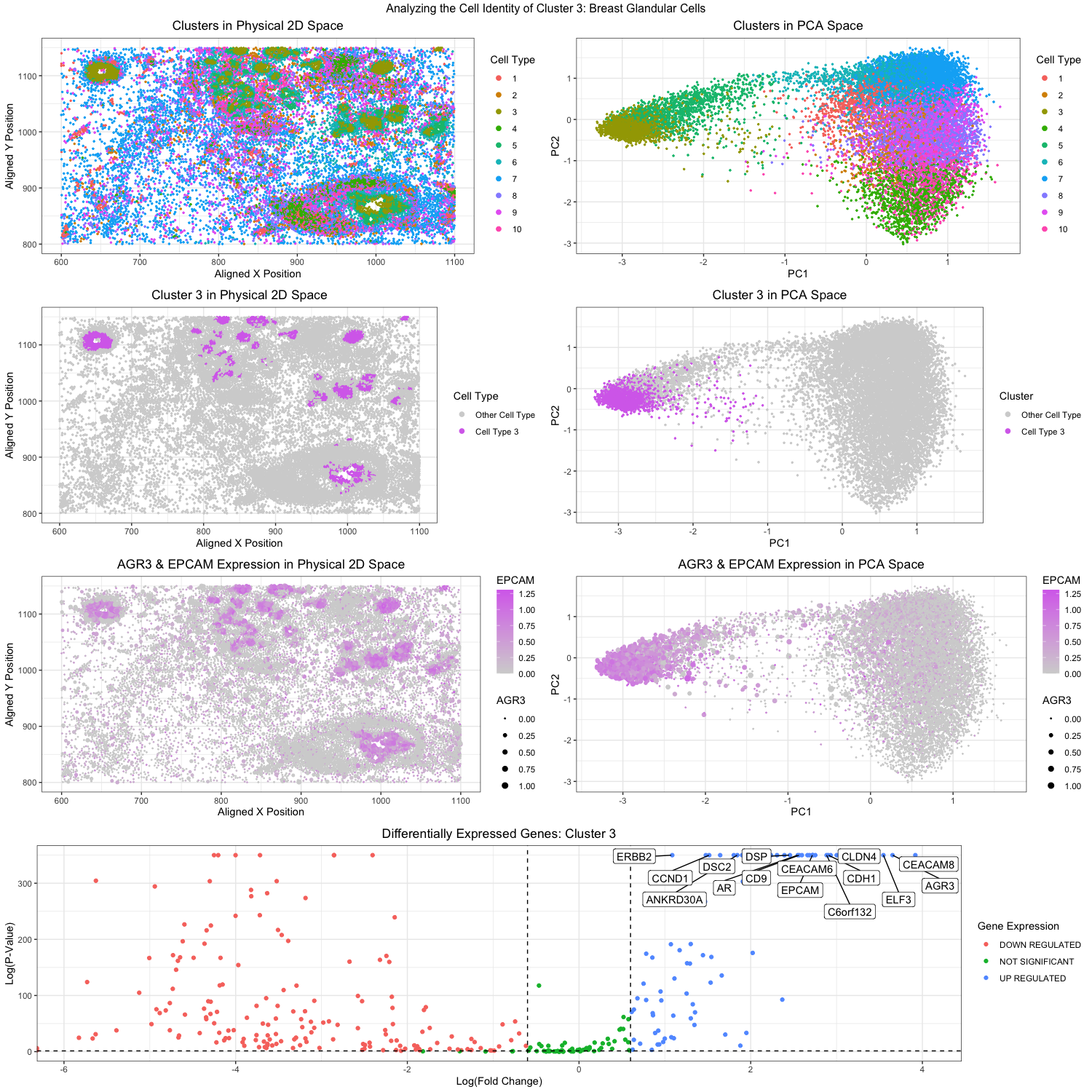
Figure Description:

In applying the workflow adapted from homework 4 (k-means clustering and differential gene expression analysis), I believe I was able to identify breast glandular cells, or more specifically, epithelial cells within the pikachu dataset. To start off, I conducted a principal component analysis on the dataset to determine that the optimal number of PCs to include in the analysis was 10. I then utilized the elbow-method to determine the optimal number of clusters to be also 10. With such information, I ran a k-means clustering on the PCs (10 PCs and 10 clusters). My analysis ultimately focused on cluster 3, which had higher expressions of EPCAM and AGR3 as visualized in the plots in the 3rd row. These visualizations proves useful below in my identification of the cell type to be breast glandular cells.

Based on the top differentially expressed genes found in cluster 3, I ultimately believe that cluster 3 contains breast glandular / epithelial cells. Such genes of interest include AGR3, CEACAM6, C6orf132, ERBB2, and EPCAM, and can be seen in the volcano plot at the very bottom. Research has identified how AGR3 expression is upregulated in breast cancer tissue, while CEACAM6 is notably expressed in several other cancers on epithelial cells [1,2]. C6orf132 has been shown to promote the proliferation of breast cancer [3]. ERBB2 is another extremely well studied breast cancer marker, and EPCAM (or Epithelial Cell Adhesion Molecule) is notably found on epithelial cells within breast carcinomas [4,5]. Looking at the protein atlas too (https://www.proteinatlas.org/), all 5 genes are linked pretty highly to breast glandular cells.

Changes in Method / Workflow:

A noticeable change in the workflow from homework 4 was the preliminary identification for the cluster of interest. In homework 4, I randomly chose a cluster to analyze, but in homework 5, because I was specifically looking to identify breast glandular cells / epithelial cells, I could not just randomly choose. So rather than just iteratively try all 10 clusters within the pikachu dataset, I decided to try a bit of “educated guessing”. I took the top 20 genes upregulated in the cluster identified from the eevee dataset containing breast glandular cells (CGN, EPS8L1, FAM83B, KRT80, FAM3B, TMPRSS2, AGR3, RIPK4, POF1B, FAM83E, SCNN1A, MYH14, RASSF6, BSPRY, ESRP2, BICDL2, ARHGEF16, CDS1, CACNG4, IRX5), and decided to see which of the genes were present in the pikachu dataset. I had hopefully expected at least 5 of the 20 genes to be present, but sadly only AGR3 was present. Luckily though, when I plotted the expression of AGR3 in the PCA space, I realized that it was pretty significantly upregulated in one cluster. That cluster would be cluster 3, and this would ultimately provide the cluster of interest I would later conclude to also be containing breast glandular cells.

Another change I introduced was for the eevee dataset, I had originally utilized the first 9 principal components (PCs) to perform the k-means clustering. However, for the pikachu dataset, I realized that the 10th PC was needed to help capture more variance in the data. This was further verified with scree plots. I think that more PCs are needed to help capture the variance in the pikachu dataset compared to the eevee dataset because there is potentially an increased diversity in the cell types captured in the pikachu dataset. Comparing the size of the eevee datasets and pikachu datasets, it can be noted that even though pikachu has significantly less genes captured (318 for pikachu v.s. 18,088 for eevee), there are significantly more “data points” captured (17,135 for pikachu v.s. 709 for eevee). This ultimately makes sense if we remember that the eevee dataset is captured with spatial beads (that group cells together) while the pikachu dataset is captured on the single-cell level. And it is this significantly increased level of distinct data points captured that I believe justifies the need for more PCs to capture the variance of the pikachu dataset.

Links / Other References:

[1] 10.1371/journal.pone.0122106

[2] 10.1111/cas.13437

[3] 10.3389/fgene.2021.636392

[4] 10.1097/01.fpc.0000166822.66754.c6

[5] 10.1016/j.talanta.2022.123715

## Packages for graphing
library(ggplot2)
library(dplyr)
library(gridExtra)
library(ggrepel)

## Packages for determining optimal cluster number
library(factoextra)
library(NbClust) 
library(cluster)

## Load the data
data <- read.csv('pikachu.csv.gz', row.names = 1)

## Isolate columns of interest
pos <- data[,4:5]
gexp <- data[,6:ncol(data)]

## Isolate cells that have gene Expression
good_cells <- rownames(gexp)[rowSums(gexp) > 0]
pos <- pos[good_cells,]
gexp <- gexp[good_cells,]

## Normalize the data
tot_gexp <- rowSums(gexp)
norm_gexp <- gexp/tot_gexp * median(tot_gexp)
log_norm_gexp <- log10(norm_gexp + 1)

## Run PCA on the data
pcs <- prcomp(log_norm_gexp)

## Determine optimal number of PCs to run for kMeans
plot(1:50, pcs$sdev[1:50], type = 'l')
plot(1:20, pcs$sdev[1:20], type = 'l')
plot(1:10, pcs$sdev[1:10], type = 'l')

## Appears that having 10 PCs is enough to account for most
## of the variance in the data.
optimal_pc_num <- 10

## Set seed for reproducibility
set.seed(1)

## Determine the optimal number of k's (centroids) for kMeans
withinnes_list <- sapply(c(5:15), function(k) { 
  tmp = kmeans(log_norm_gexp, centers = k)
  return(tmp$tot.withinss)} )

elbow <- ggplot(data.frame(k = c(5:15), tot_withinss = withinnes_list), aes(k, tot_withinss)) +
  geom_point()

elbow

## Identifying optimal number of k's
optimal_k <- 10 

## Run kMeans
cluster_pcs <- kmeans(pcs$x[,1:optimal_pc_num], centers = optimal_k)
df_cluster <- data.frame(pos, cell_type = as.factor(cluster_pcs$cluster), log_norm_gexp, pcs$x[,1:optimal_k])

## Visualizing cells in the 2D space
clusters_2D <- ggplot(data = df_cluster, aes(x = aligned_x, y = aligned_y, col = cell_type)) + 
  geom_point(size = 0.5) + 
  theme_bw() +
  theme(plot.title = element_text(hjust = 0.5)) +
  xlab("Aligned X Position") + ylab("Aligned Y Position") +
  guides(color = guide_legend(override.aes = list(size = 2))) +
  labs(title = 'Clusters in Physical 2D Space', col = "Cell Type")

clusters_2D

## Visualizing cells in the PCA space
clusters_PCA <- ggplot(data = df_cluster, aes(x = PC1, y = PC2, col = cell_type)) + 
  geom_point(size = 0.5) + 
  theme_bw() + 
  theme(plot.title = element_text(hjust = 0.5)) +
  guides(color = guide_legend(override.aes = list(size = 2))) +
  labs(title = 'Clusters in PCA Space', col = "Cell Type")

clusters_PCA

## Previous top 20 genes are contained within previous_gene_list
previous_gene_list <- list("CGN", "EPS8L1", "FAM83B", "KRT80", "FAM3B", "TMPRSS2", "AGR3", "RIPK4", "POF1B", "FAM83E", "SCNN1A", "MYH14", "RASSF6", "BSPRY", "ESRP2", "BICDL2", "ARHGEF16", "CDS1", "CACNG4", "IRX5")
for (gene in previous_gene_list) {
  # Check if the gene exists as a column name in df_cluster
  if (gene %in% colnames(df_cluster)) {
    print(gene)
  }
}

## Out of the 20 genes, only AGR3 appears :( 
## Going to pivot to looking at most expressed genes in Breast Glandular Cells from https://www.proteinatlas.org/
atlas_gene_list <- list("AQP5", "ATP6V0A4", "TMEM213", "AQP2", "AQP6", "CALM5", "GPR12", "OTX1")
for (gene in atlas_gene_list) {
  # Check if the gene exists as a column name in df_cluster
  if (gene %in% colnames(df_cluster)) {
    print(gene)
  }
} ## No genes from protein atlas show up :(

## Going to see where "AGR3" is highly expressed
agr3_PCA <- ggplot(data = df_cluster, aes(x = PC1, y = PC2, col = AGR3)) +
  geom_point(size = 0.5) + 
  theme_bw() + 
  scale_color_gradient(low = 'lightgrey', high = 'blue') + 
  labs(x = "Aligned X Position", y = "Algned Y Position", color = "AGR3", title = "AGR3 Expression in PCA Space") + 
  theme(plot.title = element_text(hjust = 0.5)) 

agr3_PCA ## Looks like expression is highest in cluster 3

## Select cluster 3 to do more analysis (confirm if it's Glandular) 

## Visualizing Cluster 3 in the 2D Space
cluster3_2D <- ggplot(data = df_cluster, aes(x = aligned_x, y = aligned_y, col = cell_type == 3)) + 
  geom_point(size = 0.5) + 
  theme_bw() +
  theme(plot.title = element_text(hjust = 0.5)) +
  guides(color = guide_legend(override.aes = list(size = 2))) +
  labs(title = 'Cluster 3 in Physical 2D Space') +
  xlab("Aligned X Position") + ylab("Aligned Y Position") +
  scale_color_manual(name = 'Cell Type',
                    values = c('lightgrey', '#D772EC'),
                    labels = c('Other Cell Type', 'Cell Type 3'))
 
cluster3_2D

## Visualizing Cluster 3 in the PCA Space
cluster3_PCA <- ggplot(data = df_cluster, aes(x = PC1, y = PC2, col = cell_type == 3)) + 
  geom_point(size = 0.5) + 
  theme_bw() + 
  theme(plot.title = element_text(hjust = 0.5)) +
  guides(color = guide_legend(override.aes = list(size = 2))) +
  labs(title = 'Cluster 3 in PCA Space') +
  scale_color_manual(name = 'Cluster',
                     values = c('lightgrey', '#D772EC'),
                     labels = c('Other Cell Type', 'Cell Type 3'))

cluster3_PCA
 
## Distinguishing between cells that are & are not within Cluster 3
cluster3 <- df_cluster[df_cluster$cell_type == 3, ]
not_cluster3 <- df_cluster[df_cluster$cell_type != 3, ]

## Identifying differentially expressed genes w/in Cluster 3 w/ Wilcox Rank Test
interest_genes <- sapply(colnames(gexp), function(g){ 
  wilcox.test(log_norm_gexp[row.names(cluster3), g], 
              log_norm_gexp[row.names(not_cluster3), g])$p.value  
})
 
## Calculating log(fold_change) for Cluster 3 --> to generate volcano plot
log_fc <- sapply(colnames(gexp), function(g) {
   log2( mean(log_norm_gexp[row.names(cluster3), g]) 
         / mean(log_norm_gexp[row.names(not_cluster3), g])) ## do ratio (log_2(A/B))
})
 
volcano <- data.frame(log_fc, log_p_val = ifelse(is.infinite(-log10(interest_genes)), 350, -log10(interest_genes)))
genes_upregulated <- sapply(colnames(gexp), function(g){
  wilcox.test(log_norm_gexp[row.names(cluster3), g], 
             log_norm_gexp[row.names(not_cluster3), g], 
             alternative = 'greater')$p.value
})
 
top_15_genes <- sort(genes_upregulated, decreasing = FALSE)[1:15]
top_15_genes

## For coloring in the points for volcano plot
volcano$diff_express <- "NOT SIGNIFICANT"
volcano$diff_express[volcano$log_fc > 0.6 & volcano$log_p_val > -log10(0.05)] <- "UP REGULATED"
volcano$diff_express[volcano$log_fc < -0.6 & volcano$log_p_val > -log10(0.05)] <- "DOWN REGULATED"

## Creating volcano plot to visualize upregulated genes in Cluster 5! 
volcano_plot <- ggplot(volcano) + 
  geom_point(aes(x = log_fc, y = log_p_val, col = diff_express)) +
  geom_vline(xintercept = c(-0.6, 0.6), linetype = 'dashed') + 
  geom_hline(yintercept=-log10(0.05), linetype = 'dashed') +
  geom_label_repel(data= volcano[names(top_15_genes),],
                   aes(x = log_fc, y = log_p_val, label = names(top_15_genes)), 
                   max.overlaps = 40, nudge_x = .05) +
  theme_bw() + 
  labs(title = 'Differentially Expressed Genes: Cluster 3',
       x = 'Log(Fold Change)', y = 'Log(P-Value)', col = "Gene Expression") + 
  theme(plot.title = element_text(hjust = 0.5))

volcano_plot

## Plot the top 2 most significant genes (AGR3, EPCAM)

## Plotting in Physical 2D Space
gene_2d <- ggplot(data = data, aes(x = aligned_x, y = aligned_y, col = EPCAM, size = AGR3)) +
  geom_point() + 
  theme_bw() + 
  scale_color_gradient(low = 'lightgrey', high = '#D772EC') + 
  scale_size(range = c(0.25, 2.5)) + 
  labs(x = "Aligned X Position", y = "Algned Y Position", size = "AGR3", color = "EPCAM", title = "AGR3 & EPCAM Expression in Physical 2D Space") + 
  theme(plot.title = element_text(hjust = 0.5)) 

gene_2d

## Plotting in PCA Space
gene_pca <- ggplot(data = df_cluster, aes(x = PC1, y = PC2, col = EPCAM, size = AGR3)) +
  geom_point() + 
  theme_bw() + 
  scale_color_gradient(low = 'lightgrey', high = '#D772EC') + 
  scale_size(range = c(0.25, 2.5)) +
  labs(size = "AGR3", color = "EPCAM", title = "AGR3 & EPCAM Expression in PCA Space") + 
  theme(plot.title = element_text(hjust = 0.5)) 

gene_pca

## Combining all the plots together
lay <- rbind(c(1,2),
             c(3,4),
             c(5,6),
             c(7,7))

grid.arrange(clusters_2D, clusters_PCA,
             cluster3_2D, cluster3_PCA,
             gene_2d, gene_pca,
             volcano_plot,
             layout_matrix = lay,
             top = "Analyzing the Cell Identity of Cluster 3: Breast Glandular Cells")

## References:
## (1) To determine the optimal number of clusters
## https://medium.com/@chyun55555/how-to-find-the-optimal-number-of-clusters-with-r-dbf84588388b 
## (2) Graphing volcano plots
## https://biocorecrg.github.io/CRG_RIntroduction/volcano-plots.html