Identifying Mammary Epitheial Cells in the Eevee Data

Write a description to convince me you found the same cell-type

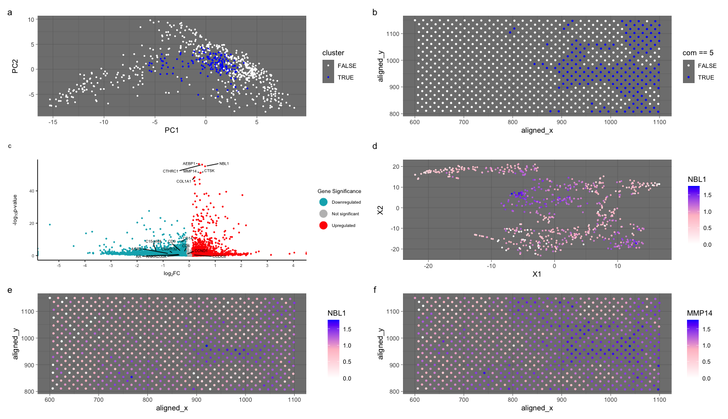
My figure features cluster 5 and links the expression of a known breast cancer gene in mammary epithelial cells to cluster 5. Further investigation showed three genes expressed in mammary epithelial cells: NBl1, MMP14, and CTSK.

I clustered the Eevee data set into 5 clusters and then chose a cluster based on the expression of gene CDH1, which is a known gene linked to breast cancer, just like in HW 4. Then, I looked for differentially expressed genes in mammary cells and cluster 5. All three genes are expressed in mammary epithelial cells. In a few resources, I discovered that NBL1 is linked to tumors associated with breast cancer. MMP14 and CTSK are highly expressed in mammary cells. As the figures show, the genes are active within the cells, upregulated, and upregulated in a few clusters. There is a higher spatial expression in cluster 5. However, it is less clear-cut than the Pikachu data set. I believe the lower expression surrounding the high expression of these genes is acceptable to classify as mammary epithelial cells because this is spatial barcode bead capture data. Other literature has classified these genes as being fibroblast cells. However, I looked for other genes known to be mammary cells, and those genes were most abundant in cluster 5. I have identified mammary cells by linking three known epithelial genes to a breast cancer gene in the same cluster and confirming with literature that these genes are expressed in mammary epithelial cells. To further validate my conclusion, I also know the cells came from breast cancer tissue.

Write a description of what you changed and why you think you had to change it.

I switched from the Pikachu to the Eevee dataset. I previously performed k-means clustering with 7 clusters. I performed k-means clustering with 5 clusters because I found the optimal K based on total withinness to be only 5 for this dataset. I think there is a lower optimal number of transcriptionally distinct cell clusters in the spot-based Eevee dataset compared to the single-cell resolution Pikachu dataset because this spatial barcode bead capture data. Multiple cells can be in one circle, reducing the number of clusters. I also adjusted the volcano plot to have a larger window for downregulation and upregulation because I was wrong to make a small window in the Pikachu dataset. I also took some code from Caleb to fix my legend in my volcano plot and adjust how I get the gene names to label my points in the volcano plot.

Sources: https://www.ncbi.nlm.nih.gov/pmc/articles/PMC9703640/ https://www.proteinatlas.org/ENSG00000157227-MMP14/tissue/breast https://www.ncbi.nlm.nih.gov/pmc/articles/PMC2630242/ https://www.proteinatlas.org/ENSG00000143387-CTSK/tissue https://www.ncbi.nlm.nih.gov/pmc/articles/PMC9053804/

library(ggplot2)
library(gridExtra)
library(Rtsne)
library(ggrepel)
library(patchwork)

data <- read.csv('~/Documents/genomicsDataVisualization/eevee.csv.gz', row.names = 1)
gexp <- data[, 4:ncol(data)]
rownames(gexp) <- data$barcode
pos <- data[2:3]

gexpnorm <- log10(gexp/rowSums(gexp) * mean(rowSums(gexp)) + 1)

#pca
pcs <- prcomp(gexpnorm)
emb <- Rtsne(pcs$x[, 1:20])$Y

# kmeans 
com <- as.factor(kmeans(gexpnorm, centers = 5)$cluster) # changed

# visualize clusters
p7 <- ggplot(data.frame(emb,com)) + 
  geom_point(aes(x = X1, y = X2, col = com), size = 0.5) + 
  theme_bw()

# cluster of interest com == 5
# other g I tested GJB2, CLDN7, CLDN19 as known mammary epithelial cells 
g <- 'CDH1' # known cancer gene 
results <- sapply(unique(com), function(i) {
  wilcox.test(gexpnorm[com == i, g],
              gexpnorm[com != i, g],
              alternative = "greater")$p.val
})
head(sort(results, decreasing=FALSE))

unique(com) # find which value corresponds to which cluster

g <- 'CDH1'
results <- sapply(colnames(gexpnorm), function(g) {
  wilcox.test(gexpnorm[com == 5, g],
              gexpnorm[com != 5, g],
              alternative = "greater")$p.val
})
head(sort(results, decreasing=FALSE)) # showed which cluster was expressed highly of gene 

# AEBP1       CTHRC1        MMP14         NBL1       COL1A1         CTSK 
# 1.684465e-60 1.347756e-59 5.792964e-57 1.013317e-49 2.402690e-49 9.951574e-49 

pcsNorm <- prcomp(gexpnorm, center = TRUE, scale = FALSE)
df <- data.frame(pcsNorm$x[, 1:15], cluster = com == 5)
p1 <- ggplot(df) + 
  geom_point(aes(x = PC1, y = PC2, col = cluster), size = 0.5) + 
  theme_dark() +
  scale_color_manual(values = c("white", "blue")) 

# cluster 5 in physical space
p2 <- ggplot(data) + geom_point(aes(x = aligned_x, y = aligned_y, col = com == 5), size = 0.8) + 
  theme_dark() +
  scale_color_manual(values = c("white", "blue"))

# volcano differentially expressed genes in cluster 3 
pv <- sapply(colnames(gexpnorm), function(i) {
  wilcox.test(gexpnorm[com == 5, i], gexpnorm[com != 5, i])$p.val
})
logfc <- sapply(colnames(gexpnorm), function(i) {
  log2(mean(gexpnorm[com == 5, i])/mean(gexpnorm[com != 5, i]))
})

# volcano plot
# https://biostatsquid.com/volcano-plots-r-tutorial/ used code from here
# got assistance from copiolt to get the labels correct 

df <- data.frame(pv=-log10(pv + 10e-300), logfc) # adjust by the 300 bc most points are inf
df$geneNames <-rownames(df) # changed 
df$diffexpressed <- "NO"
df$diffexpressed[df$logfc > .1 ] <- "UP" # changed
df$diffexpressed[df$logfc < -.1] <- "DOWN" # changed
genes_of_interest <- c("CLDN19", "CD4","CCND1", "AGR3", "ANKRD30A", "C6orf132", "CD14", "CD9", "CCDC6", "C15orf48", "AR","AEBP1", "CTHRC1", "MMP14", "NBL1", "COL1A1", "CTSK")
df$label <- ifelse(rownames(df) %in% genes_of_interest, rownames(df), NA)
p3 <- ggplot(df, aes(x = logfc, y = pv, col = diffexpressed, label = label)) + 
  geom_point(size = 0.5, key_glyph = "point") + 
  scale_color_manual(values = c("#00AFBB", "grey", "red"),
                     labels = c("Downregulated", "Not significant", "Upregulated")) +
  # theme
  theme_classic() +
  # labels
  labs(color = 'Gene Significance', 
       x = expression("log"[2]*"FC"), 
       y = expression("-log"[10]*"p-value"),
       title = "") +
  theme(
    plot.title = element_text(hjust = 0.5, face="bold", size=10),
    text = element_text(size = 8)
  ) + 
  geom_text_repel(max.overlaps = Inf, box.padding = 0.25, point.padding = 0.25, min.segment.length = 0, size = 2, color = "black") + 
  scale_x_continuous(breaks = seq(-5, 5, 1)) +
  guides(size = "none",color = guide_legend(override.aes = list(size=5)))

gene <- AEBP1
# Rtsne space of differentially expressed gene
p4 <- ggplot(data.frame(emb, NBL1 = gexpnorm[, 'NBL1'])) + 
  geom_point(aes(x = X1, y = X2, col = NBL1), size = 0.5) + 
  scale_colour_gradient2(low = 'white', mid = 'pink', high = 'blue', midpoint = max(gexpnorm[, 'NBL1'])/2) + theme_dark()

# gene in physical space
p5 <- ggplot(data.frame(pos, gexpnorm)) + 
  geom_point(aes(x = aligned_x, y = aligned_y, col = NBL1), size = 0.9) + 
  scale_colour_gradient2(low = 'white', mid = 'pink', high = 'blue', midpoint = max(gexpnorm[, 'NBL1'])/2) + 
  theme_dark()

p6 <- ggplot(data.frame(pos, gexpnorm)) + 
  geom_point(aes(x = aligned_x, y = aligned_y, col = MMP14), size = 0.9) + 
  scale_colour_gradient2(low = 'white', mid = 'pink', high = 'blue', midpoint = max(gexpnorm[, 'MMP14'])/2) + 
  theme_dark()
p1 + p2 + p3 + p4 + p5 + p6 + plot_annotation(tag_levels = 'a') + plot_layout(ncol = 2)