Identifying KRT8 Expression in Spot-Based Spatial Transcriptomic Data Set

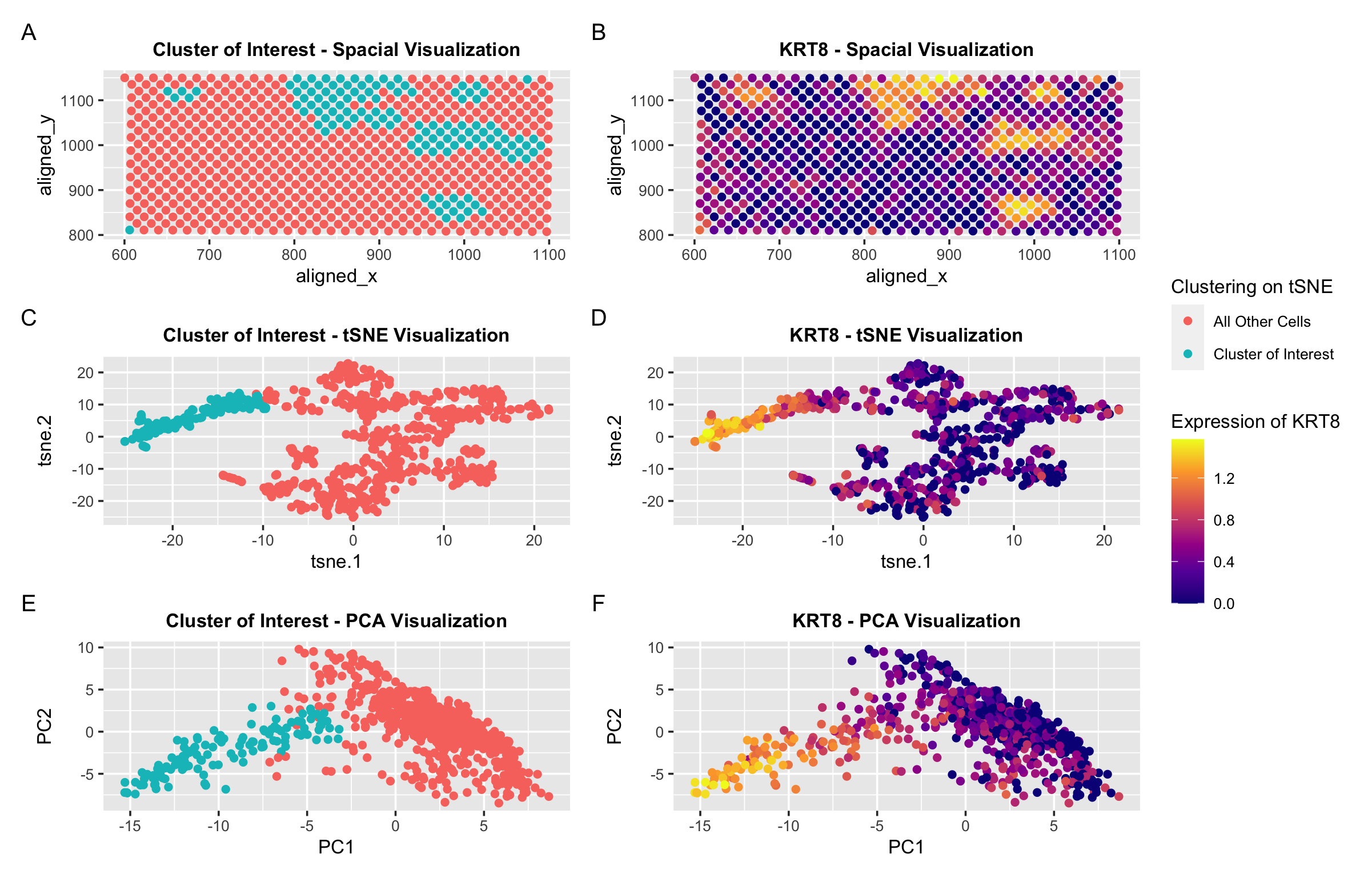
In the pikachu Single Cell Data Set, I identified a cluster of cells that had high expression of the KRT8 gene. I hypothesized that these cells were epithelial cells.
In my orginial investigation, I found that the KRT8 gene was almost exclusively upregulated in the cell cluster I identified. Thus, I used expression of this gene to identify a similar cluster of spots in the same general spatial location and pattern with similar upregulation of the KRT8 gene. Panels A and B show the spatial location of the spots of interest as well as the gene expression. Panels C and D show the lower dimension tSNE embedding. And finally, Panels E and F show the lower dimension PCA graph.
I made slight modifications to my code to identify this cluster. In addition to adjusting which columns I extracted data from, I also used a different k for k-means clustering. I previously performed k-means clustering with k=5. Now I performed k-means clustering with k=4. This is because I found the optimal K based on total withinness to be 4. While the cluster of interest was usually isolated with many different values of k, I found that higher k values seemed to oversegment the other cells. I think there is a lower optimal number of transcriptionally distinct cell-clusters in the spot-based Eevee dataset compared to the single-cell resolution Pikachu dataset because many cells may be in a single spot. Thus, it may be more difficult to identify/distinguish between distinct cell types.
#HW5
#Andrea Cheng (acheng41)

data = read.csv("~/Desktop/GDV class/data/eevee.csv.gz", row.names =1)

#import libraries
library(Rtsne)
library(ggplot2)
library(patchwork)

#design of visualization
my_color = scale_color_viridis_c(option= "C")
my_theme = theme(
  plot.title = element_text(hjust = 0.5, face="bold", size=10),
  text = element_text(size = 10)
)


data[1:5,1:10]
pos = data[,2:3]
head(pos)
gexp = data[,4:ncol(data)]

#normalize
gexpnorm = log10(gexp/rowSums(gexp) * mean(rowSums(gexp)) + 1)


#identify cell cluster
df_plot = data.frame(pos, gene = gexpnorm[,'KRT8'])
#plot on tissue
gene_tissue = ggplot(df_plot) +
  geom_point(aes(x=aligned_x, y = aligned_y,
                 col = gene)) + my_color +
  labs(col = "Expression of KRT8",
       title = "KRT8 - Spacial Visualization")+ my_theme

#PCA
pcs = prcomp(gexpnorm)
plot(pcs$sdev[1:20])

#tsne
emb = Rtsne(pcs$x[,1:20])$Y #faster w/ pcs which represent genes than tSNE on genes
df_tsne = data.frame(emb)
#check tsne plot
ggplot(df_tsne) + geom_point(aes(x = X1, y = X2)) + theme_classic()


#find optimal clustering coefficient k on tSNE
#look at different tot.within-ness for different k
results <- sapply(2:15, function(i){
  com <- kmeans(emb, centers = i)
  return(com$tot.withinss)
})
plot(results, type = 'l')


#kmeans with k=4
com = kmeans(emb, centers = 4)

#visualize clusters
df_clusters = data.frame(pos, tsne = emb, pcs = pcs$x, kmeans = as.factor(com$cluster))

#Plot showing cluster of interest in tSNE
kmeans_tsne = ggplot(df_clusters) +
  geom_point(aes(x=tsne.1,y = tsne.2,
                 col = ifelse(kmeans == 3, "Cluster of Interest", "All Other Cells"))) +
  labs(
    col = "Clustering on tSNE",
    title = "Cluster of Interest - tSNE Visualization"
  ) + my_theme

#Plot showing cluster of interest in tissue
kmeans_tissue = ggplot(df_clusters) +
  geom_point(aes(x=aligned_x,y = aligned_y,
                 col = ifelse(kmeans == 3, "Cluster of Interest", "All Other Cells")))+
  labs(
    col = "Clustering on tSNE",
    title = "Cluster of Interest - Spacial Visualization"
  )+ my_theme

#Plot showing cluster of interest in PCA
kmeans_pca = ggplot(df_clusters) +
  geom_point(aes(x=pcs.PC1,y = pcs.PC2,
                 col = ifelse(kmeans == 3, "Cluster of Interest", "All Other Cells"))) +
  labs(
    col = "Clustering on tSNE",
    title = "Cluster of Interest - PCA Visualization"
    ) + xlab("PC1") +  ylab ("PC2") + my_theme

#data frame for gene expression of KRT8
df_gene = data.frame(pos, tsne = emb, pcs = pcs$x, gene = gexpnorm$KRT8)

#Plot showing gene expression in tSNE
gene_tsne = ggplot(df_gene) + geom_point(aes(x = tsne.1, y=tsne.2, col = gene)) +
  my_color + labs(
    col = "Expression of KRT8",
    title = "KRT8 - tSNE Visualization"
  )+ my_theme

#Plot showing gene expression in PCA
gene_pca = ggplot(df_gene) + geom_point(aes(x=pcs.PC1,y = pcs.PC2, col = gene)) +
  my_color + xlab("PC1") +  ylab ("PC2") +
  labs(
    col = "Expression of KRT8",
    title = "KRT8 - PCA Visualization"
  )+ my_theme

#display plots
kmeans_tissue + gene_tissue + kmeans_tsne + gene_tsne + kmeans_pca + gene_pca + plot_annotation(tag_levels = 'A')+
  plot_layout(widths = c(5, 5, 5),
              guides = "collect",
              design = "
              12
              34
              56
              ")