Locating glandular epithelial cells within the Pikachu data

Write a description of what you changed and why you think you had to change it.
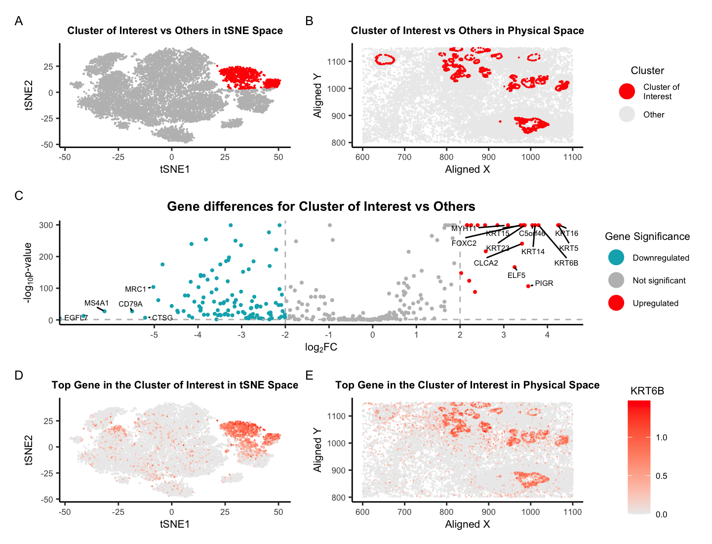
For Homework 5, I am switching from the Eevee dataset to the Pikachu dataset. I was able to successfully identify the same cell-type in the Pikachu dataset as I did in the Eevee dataset, glandular epithelial cells, with some minor tweaks to my previous Homework 4 code. Originally, I was using k-means clustering with k=5, but this time around, I cranked it up to k=12. Even though the plot of total withinness suggested ~6 clusters might be the sweet spot, I went with k=12 knowing it would help me find the same cell type I did before. Further, I believe that the Pikachu dataset, which offers single-cell resolution instead of Eevee’s spot-based approach, will allow us see more unique cell clusters because it has more observations to work with, which will likely leads to more transcriptional diversity compared to the Eevee dataset which may have multiple cell types within each spot.
Another change I made was to analyze all genes instead of just focusing on the top ones since there are only around 300 genes to consider, which isn’t as overwhelming compared to the massive list of about 18,000 genes the Eevee dataset has. To deal with the log(0) situation, I added 10e-300 to the p-value for the two-sided Wilcoxon Rank Sum test. Finally, one neat thing I did was to add layers of geom_point() so the points of interest are on the top layer. This allows for those points to be seen more easily and not be plotted underneath of unimportant points (or the gray points in this figure).
After these tweaks, I was able to find a cluster of interest that has high expression of the same gene, KRT6B [1], as the glandular epithelial cells I found in the Eevee dataset. Further, one of the other genes I found associated with this cluster, KRT23 [3], is also highly expressed within this new cluster of interest. While KRT17 [2] was not obtained in the Pikachu data, there are other genes within the KRT family, such as KRT5, that are known to be highly expressed in epithelial cells [7]. If that is not enough proof, if we overlaid the two physical space plots of the Eevee and Pikachu datasets, we would see that the cluster of interest in the Pikachu dataset is nearly in the same location as the cluster of interest in the Eevee dataset. Since the Eevee and Pikachu datasets are serial sections of the same tissue, it makes sense that I was able to find the same cell type, glandular epithelial cells, in both datasets!
Below are my references from Homework 4, giving more information about these genes and why they relate to glandular epithelial cells.
References
[1] https://www.ncbi.nlm.nih.gov/gene/3854
[2] https://www.ncbi.nlm.nih.gov/gene/3872
[3] https://www.genecards.org/cgi-bin/carddisp.pl?gene=KRT23
[4] https://www.ncbi.nlm.nih.gov/pmc/articles/PMC9496156/
[5] https://osf.io/preprints/osf/nsker
[6] https://pubmed.ncbi.nlm.nih.gov/36353580/
[7] https://www.ncbi.nlm.nih.gov/gene/3852
Code
### HW5 ###
## Caleb Hallinan ##
## Pikachu sequencing data ##

# import libraries
library(here)
library(ggplot2)
library(Rtsne)
library(patchwork)
library(factoextra)
library(ggrepel)

# set seed
set.seed(02052024)


#### Data Preprocessing ####

# read in data
data = read.csv(here("data/pikachu.csv.gz"), row.names = 1)
# dim(data)
# get info from data
pos <- data[,4:5]
gexp <- data[,6:ncol(data)]
# colnames(gexp)

# normalize log2
gexpnorm <- log10(gexp/rowSums(gexp) * mean(rowSums(gexp))+1)


#### Dimensionality Reduction ####

# perform pca
pcs <- prcomp(gexpnorm)

# run tsne on top PCs
set.seed(02052024)
emb <- Rtsne(pcs$x[,1:20], perplexity = 15) # can change dims from
# names(emb)

# gene to plot
gene <- "KRT6B" # NOTE: this was my gene of interest from HW4

# plot tsne to see
# ggplot(data.frame(emb$Y)) +
#     geom_point(aes(x = emb$Y[,1], y = emb$Y[,2], color =gexpnorm$KRT6B)) +
#     theme_classic() +
#     labs(
#         title = "tSNE on Top 1000 Genes with High Variance",
#         color = gene,
#         x = "tSNE1",
#         y = "tSNE2"
#     ) +
#     scale_color_gradient2(midpoint = median(gexpnorm[[gene]]), low = "blue", mid = "#ECECEC", high = "red", space = "Lab" ) +
#     theme(legend.title.align=0.5,plot.title = element_text(hjust = 0.5, face="bold", size=14), text = element_text(size = 13))


#### Clustering ####

#create plot of number of clusters vs total within sum of squares
# fviz_nbclust(data.frame(emb$Y), kmeans, method = "wss")

# perform kemans clustering based on elbow plot
set.seed(02052024)
clusters <- as.factor(kmeans(emb$Y, 12)$cluster)

# get just cluster of interest
cluster_of_interest <- ifelse(clusters == 6, "Cluster of\nInterest", "Other")

# plot tsne to see
ggplot(data.frame(emb$Y)) +
    geom_point(aes(x = emb$Y[,1], y = emb$Y[,2], color = clusters), size=0.75) +
    theme_classic() +
    labs(
        title = "Clusters in tSNE Space",
        color = "Cluster",
        x = "tSNE1",
        y = "tSNE2"
    ) +
    theme(legend.title.align=0.5,plot.title = element_text(hjust = 0.5, face="bold", size=8), text = element_text(size = 8))


#### DE Gene Analysis ####

# do wilcox for DE genes
pv <- sapply(colnames(gexpnorm), function(i) {
    print(i) ## print out gene name
    wilcox.test(gexpnorm[clusters == 6, i], gexpnorm[clusters != 6, i])$p.val
})

head(sort(pv))

# get log fold change
logfc <- sapply(colnames(gexpnorm), function(i) {
    print(i) ## print out gene name
    log2(mean(gexpnorm[clusters == 6, i])/mean(gexpnorm[clusters != 6, i]))
})


### Plotting ###

# gene to plot
gene <- "KRT6B" # NOTE: this was my gene of interest from HW4

# add cluster of interest to data
data$cluster_of_interest <- cluster_of_interest
# add gene of interest to data
data$gene_of_interest <- gexpnorm[[gene]]

# create df for tsne to plot layers
tsne_emb <- data.frame(emb$Y)
tsne_emb$cluster_of_interest <- cluster_of_interest
tsne_emb$gene_of_interest <- gexpnorm[[gene]]

# plot tsne to see
bottom1 <-ggplot(tsne_emb) +
    geom_point(data = tsne_emb[cluster_of_interest == "Other",], aes(x = X1, y = X2, color = gene_of_interest), size=0.01) +
        geom_point(data = tsne_emb[cluster_of_interest == "Cluster of\nInterest",], aes(x = X1, y = X2, color = gene_of_interest), size=0.01) +
        theme_classic() +
    labs(
        title = "Top Gene in the Cluster of Interest in tSNE Space",
        color = gene,
        x = "tSNE1",
        y = "tSNE2"
    ) +
    scale_color_gradient2(midpoint = median(gexpnorm[[gene]]), low = "blue", mid = "#ECECEC", high = "red", space = "Lab" ) +
    theme(legend.title.align=0.5,plot.title = element_text(hjust = 0.5, face="bold", size=8), text = element_text(size = 8)) +
    guides(color = "none")


bottom2 <- ggplot(data) +
    geom_point(data = data[cluster_of_interest == "Other",], aes(x = aligned_x, y = aligned_y, color = gene_of_interest[cluster_of_interest == "Other"]), size=0.01) +
    geom_point(data = data[cluster_of_interest == "Cluster of\nInterest",], aes(x = aligned_x, y = aligned_y, color = gene_of_interest[cluster_of_interest == "Cluster of\nInterest"]), size=0.01) +
    scale_color_gradient(low = "#ECECEC", high = "red", space = "Lab" ) +
    # scale_color_gradient2(midpoint = max(gexpnorm[[gene]])/2, low = "blue", mid = "#ECECEC", high = "red", space = "Lab" ) +
    theme_classic() +
    labs(
        title = "Top Gene in the Cluster of Interest in Physical Space",
        color = gene,
        x = "Aligned X",
        y = "Aligned Y"
    ) +
    guides(size = "none") +
    theme(legend.title.align=0.5,plot.title = element_text(hjust = 0.5, face="bold", size=8),
          text = element_text(size = 8))


top1 <- ggplot(data.frame(emb$Y)) +
    geom_point(aes(x = emb$Y[,1], y = emb$Y[,2], color = cluster_of_interest), size=0.01) +
    scale_color_manual(values = c("red","gray")) +
    theme_classic() +
    labs(
        title = "Cluster of Interest vs Others in tSNE Space",
        color = "Cluster",
        x = "tSNE1",
        y = "tSNE2"
    ) +
    # scale_color_gradient2(midpoint = median(gexpnorm[[gene]]), low = "blue", mid = "#ECECEC", high = "red", space = "Lab" ) +
    theme(legend.title.align=0.5,plot.title = element_text(hjust = 0.5, face="bold", size=8), text = element_text(size = 8)) +
    guides(color = "none")


top2 <- ggplot() +
    geom_point(data = data[cluster_of_interest == "Other",], aes(x = aligned_x, y = aligned_y, color = cluster_of_interest), size=0.01) +
    geom_point(data = data[cluster_of_interest == "Cluster of\nInterest",], aes(x = aligned_x, y = aligned_y, color = cluster_of_interest), size=0.01) +
    scale_color_manual(values = c("red","#ECECEC")) +
    # scale_color_gradient2(midpoint = max(gexpnorm[[gene]])/2, low = "blue", mid = "#ECECEC", high = "red", space = "Lab" ) +
    theme_classic() +
    labs(
        title = "Cluster of Interest vs Others in Physical Space",
        color = "Cluster",
        x = "Aligned X",
        y = "Aligned Y"
    ) +
    guides(size = "none",color = guide_legend(override.aes = list(size=5))) +
    theme(legend.title.align=0.5, plot.title = element_text(hjust = 0.5, face="bold", size=8),
          text = element_text(size = 8))


# volcano plot
df <- data.frame(pv=-log10(pv + 10e-300), logfc)
# add gene names
df$genes <- rownames(df)
# add labeling
df$delabel <- ifelse(df$logfc > 3, df$genes, NA)
df$delabel <- ifelse(df$logfc < -5, df$genes, df$delabel)
# add if DE
df$diffexpressed <- ifelse(df$logfc > 2, "Upregulated", "Not Significant")
df$diffexpressed <- ifelse(df$logfc < -2, "Downregulated", df$diffexpressed)

# plot
mid <- ggplot(df, aes(x = logfc, y = pv, label = delabel, color = diffexpressed)) +
    geom_point(size= 0.75) +
    geom_vline(xintercept = c(-2, 2), col = "gray", linetype = 'dashed') +
    geom_hline(yintercept = -log10(0.05), col = "gray", linetype = 'dashed') +
    scale_color_manual(values = c("#00AFBB", "grey", "red"),
                       labels = c("Downregulated", "Not significant", "Upregulated")) +
    # theme
    theme_classic() +
    # labels
    labs(color = 'Gene Significance',
         x = expression("log"[2]*"FC"),
         y = expression("-log"[10]*"p-value"),
         title = "Gene differences for Cluster of Interest vs Others") +
    theme(
        plot.title = element_text(hjust = 0.5, face="bold", size=10),
        text = element_text(size = 8)
    ) +
    geom_text_repel(max.overlaps = Inf, box.padding = 0.25, point.padding = 0.25, min.segment.length = 0, size = 2, color = "black") +
    scale_x_continuous(breaks = seq(-5, 5, 1)) +
    guides(size = "none",color = guide_legend(override.aes = list(size=5)))


# plot using patchwork
(top1 + top2) / (mid) / (bottom1 + bottom2) + plot_annotation(tag_levels = 'A')