Analysis of Sequencing Dataset Clustering, AGR3 Expression, and cell-typing

Description

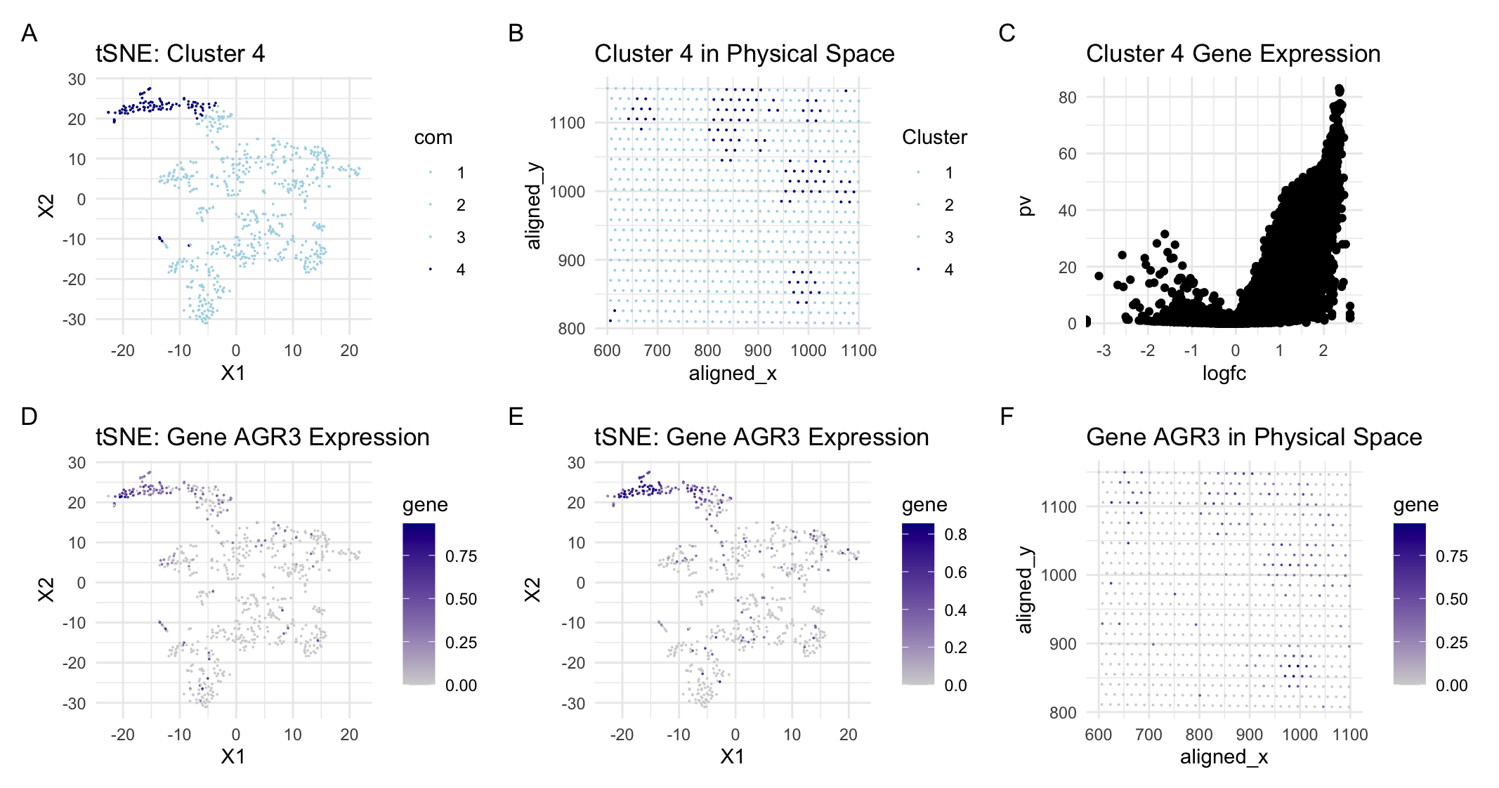
For this assignment, I switched from the Pikachu to the Eevee dataset. I previously found that most of the variation was captured by about 20 PCs following PCA. With the new dataset, most of the variation is captured within about 9 PCs. This is likely because the sequencing dataset has less variation than the imaging dataset since only the cells within the wells are sequenced and recorded in the dataset. Since there is less variation, I also performed k-means clustering with fewer clusters reducing from k=6 for the imaging dataset to k=4 for the sequencing dataset. To determine which cluster is likely to be the same cell-type (breast glandular cells) that I characterized in the previous assignment, I searched for expression of the same gene (AGR3) and matched the highest areas of AGR3 expression to cluster 4 in the sequencing dataset. Then, I analyzed cluster 4 to determine if these were in fact the same cells I categorized in the previous assignment.

The easiest way to visually confirm this was to analyze the spatial orientation of cluster 4 and the cells with high AGR3 expression. Even though the sequencing dataset only has dots, the location was about the same as it was in the imaging dataset and the cells of interest were in tight groupings just as they were in the imaging dataset. Additionally, I determined that the most expressed gene in cluster 4 was RHOV. Based on a preliminary search, RHOV when found in breast tissue is specifically expressed in breast cancer cells. This finding aligned with my previous theory that the tight groupings of cells are indicative of oncogenic cells. It also aligned with the function of AGR3 which plays a key role in the proliferation of these breast cancer cells. Given all of this, I can be reasonably sure that I have identified the same cells across the two datasets.

References

https://www.proteinatlas.org/ENSG00000104140-RHOV https://www.ncbi.nlm.nih.gov/pmc/articles/PMC6959303/ https://www.proteinatlas.org/ENSG00000104140-RHOV/pathology/breast+cancer https://www.ncbi.nlm.nih.gov/pmc/articles/PMC10236621/#:~:text=In%20the%20CCLE%20database%2C%20RhoV,cancer%20(Figure%20S2B).

## starting with the code from HW 4 and modifying it for the eevee dataset
# code credit to the class notes this past week

# libraries
library(ggplot2)
library(Rtsne)
library(patchwork)

# read in the data
data = read.csv('/Users/Kyra_1/Documents/College/Junior/Spring/Genomic_Data_Visualization/Homework_1/eevee.csv.gz', row.names = 1)
#data[1:5, 1:10]
#pos = data[, 4:5]
#gexp = data[6:ncol(data)]
pos = data[,2:3]
gexp = data[, 3:ncol(data)]
# normalize
gexpnorm = log10(gexp/rowSums(gexp) * mean(rowSums(gexp))+1)

# dimensionality reduction: PCA
pcs = prcomp(gexpnorm)
p6 = plot(pcs$sdev[1:100])
## most variation is captured by about 9 pcs
## note this is different than the pikachu dataset

# RTSNE
emb = Rtsne(pcs$x[, 1:9])$Y

# kmeans clustering
## less variation, needed fewer clusters
com = as.factor(kmeans(gexpnorm, centers = 4)$cluster)

# CLUSTER 4 contains the cell type of interest
# cluster of interest in reduced space
p1 = ggplot(data.frame(emb,com)) + geom_point(aes(x = X1, y = X2, col = com), size = 0.01)+
  scale_color_manual(values = c("lightblue", "lightblue", "lightblue", "darkblue"))+
  labs(title = "tSNE: Cluster 4")+
  theme_minimal()

# cluster of interest in physical space
p2 = ggplot(data.frame(pos, Cluster = com)) + 
  geom_point(aes(x= aligned_x, y = aligned_y, col = Cluster), size = 0.05)+
  scale_color_manual(values = c("lightblue", "lightblue", "lightblue", "darkblue"))+
  labs(title = "Cluster 4 in Physical Space")+ theme_minimal()

# volcano plots to visualize differentially expressed genes in the cluster of interest
pv = sapply(colnames(gexp), function(i){
  wilcox.test(gexp[com ==4, i], gexp[com != 4, i])$p.val
})

logfc = sapply(colnames(gexp), function(i){
  ## if this mean is exactly 1, then the means are equal across the population
  log2(mean(gexp[com == 4, i])/mean(gexp[com != 1, i]))
})

p3 = ggplot(data.frame(pv = -log10(pv), logfc))+ geom_point(aes(x = logfc, y = pv))+
  labs(title = "Cluster 4 Gene Expression")+ theme_minimal()

# picking a gene:
# find the most differentially expressed gene in each cluster
results2 <- sapply(1:4, function(i){
  print(i)
  results = sapply(colnames(gexpnorm), function(g){
    wilcox.test(gexpnorm[com == i, g],
                gexpnorm[com != i, g], 
                alternative = "greater")$p.val
  })
  topgene = names(head(sort(results, decreasing= F))[1])
  print(topgene)
  return(topgene)
})

# 'AGR3' is the most expressed gene in the fourth cluster
# pick a cluster of interest: CLUSTER 4
g = 'AGR3'
gexpnorm[com == 4, g]
gexpnorm[com != 4, g]
par(mfrow=c(2,1))
hist(gexpnorm[com == 4, g])
hist(gexpnorm[com != 4, g])

# run a t-test
t.test(gexpnorm[com == 4, g], gexpnorm[com != 4, g], alternative = "two.sided")$p.val

# visualizing the gene in reduced dimensional space
p4 = ggplot(data.frame(emb, gene = gexpnorm[, 'AGR3'])) + 
  geom_point(aes(x = X1, y = X2, col = gene), size = 0.01)+
  scale_color_gradient2(high = 'darkblue', mid = 'lightgrey', low = 'lightblue')+
  labs(title = "tSNE: Gene AGR3 Expression")+ theme_minimal()

# visualizing the gene in space
## need to modify the data frame still
p5 = ggplot(data.frame(pos, gene = gexpnorm[, 'AGR3'])) + 
  geom_point(aes(x=aligned_x, y = aligned_y, col = gene), size = 0.01)+
  scale_color_gradient2(high = 'darkblue', mid = 'lightgrey', low = 'lightblue')+
  labs(title = "Gene AGR3 in Physical Space")+ theme_minimal()

# visualizing the gene in reduced dimensional space
p6 = ggplot(data.frame(emb, gene = gexpnorm[, 'RHOV'])) + 
  geom_point(aes(x = X1, y = X2, col = gene), size = 0.01)+
  scale_color_gradient2(high = 'darkblue', mid = 'lightgrey', low = 'lightblue')+
  labs(title = "tSNE: Gene AGR3 Expression")+ theme_minimal()


# stitch the graphs together using patchwork
p1 + p2 + p3 + p4 + p6 + p5 + plot_annotation(tag_levels = 'A')