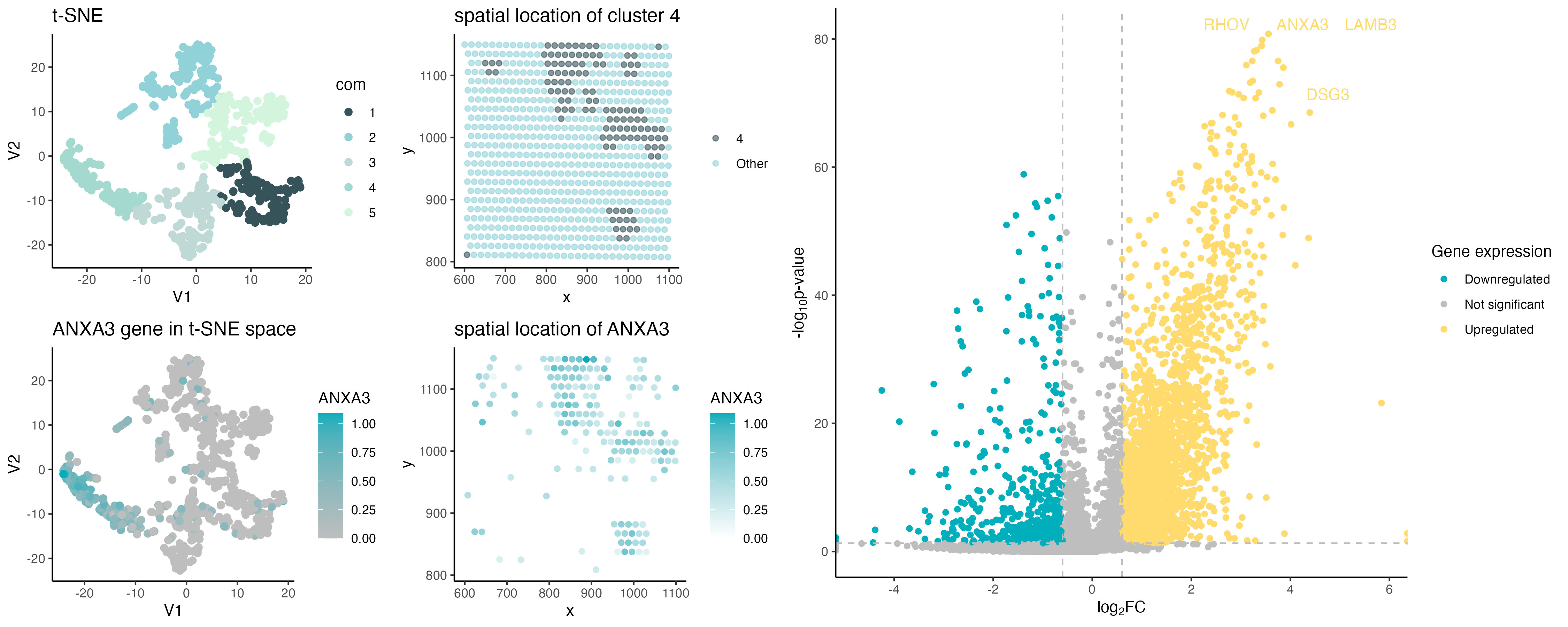
ANXA3 spatial expression

Code changes from pikachu to eevee dataset
t-SNE optimization based on elbow plot
t-SNE was run on 10 PCs rather than 50 PCs due to the elbow plot showing variance plateau at 10 PCs. By using fewer components, it simplifies dimensionality reduction while still being able to capture most variance.
Adapt to the specific genes present in the dataset
The gene CD8B was replaced with ANXA3 as it was not present in the eevee dataset. ANXA3 gene was chosen as it showed significant upregulation of this gene in cluster 4.
Optimize spatial plots for spot-based data
The dot size was increased because the eevee data is spot-based instead of the pikachu single cell dataset, allowing more whitespace to visualize larger dots.
References
https://biostatsquid.com/volcano-plots-r-tutorial/ https://cran.r-project.org/web/packages/gridExtra/vignettes/arrangeGrob.html
#### author ####
# Andre Forjaz
# jhed: aperei13

#### load packages ####
library(Rtsne)
library(ggplot2)
library(patchwork)
library(gridExtra)
library(umap)
library(ggrepel)
library(tidyverse)
library(RColorBrewer)
#### Input ####
outpth <-'~/Documents/genomics data visualization 2024 course/homework/hw5/'
pth <-'~/Documents/genomics data visualization 2024 course/data/eevee.csv.gz'
data <- read.csv(pth, row.names=1)
# pick color palette
colpal <- c("#365359", "#91D2D9", "#BFD9D6", "#A3D9CF","#D4F5DD", "#F2F2F2")

# data preview
data[1:5,1:8]

# xy data
pos <- data[, 2:3]
# gene data
gexp <- data[4:ncol(data)]
# normalize the data with log10 mean
gexpnorm <- log10(gexp/rowSums(gexp) * mean(rowSums(gexp))+1)

rownames(pos) <- rownames(gexpnorm) <- data$cell_id
head(pos)
head(gexp)

# PCA
pcs <- prcomp(gexpnorm)
plot(pcs$sdev[1:50])

# tsne on pcs
emb <- Rtsne::Rtsne(pcs$x[,1:10])$Y
plot(emb)

# identify clusters kmeans
com <- as.factor(kmeans(emb, centers = 5)$cluster)

## Panel A
# tsne visualization
df_a <- data.frame(V1 = emb[,1],
                   V2 = emb[,2],
                   cluster = com)

pa <- ggplot(df_a) +
  geom_point(aes(V1, V2, color=com),size = 2) +
  scale_color_manual(values = colpal[])+
  ggtitle("t-SNE")+
  theme_classic()

pa

## Panel B
# spatial resolved cluster
df_b <- data.frame(x = pos$aligned_x,
                   y = pos$aligned_y,
                   cluster = com)
cluster_nr <-4
pb <- ggplot(df_b) +
  geom_point(aes(x, y,
                 color= ifelse(cluster == cluster_nr, "4", "Other")),
             size =1.5,
             alpha = 0.6) +
  scale_color_manual(values = colpal, guide = guide_legend(title = NULL))+
  ggtitle("spatial location of cluster 4")+
  theme_classic()

pb

## Panel C
# differentially expressed genes for your cluster of interest
pv <- sapply(colnames(gexpnorm), function(i) {
  # print(i) ## print out gene name
  wilcox.test(gexpnorm[com == cluster_nr, i], gexpnorm[com != cluster_nr, i])$p.val
})

logfc <- sapply(colnames(gexpnorm), function(i) {
  # print(i) ## print out gene name
  log2(mean(gexpnorm[com == cluster_nr, i])/mean(gexpnorm[com != cluster_nr, i]))
})

# volcano plot
df_c <- data.frame(pv=pv, logfc,gene_symbol=colnames(gexpnorm))
# Credit: https://biostatsquid.com/volcano-plots-r-tutorial/
df_c$diffexpressed <- "NO"
# Set as "UP" if log2Foldchange > 0.6 and pvalue < 0.05
df_c$diffexpressed[df_c$logfc > 0.6 & df_c$pv < 0.05] <- "UP"
# Set as "DOWN" if log2Foldchange < -0.6 and pvalue < 0.05
df_c$diffexpressed[df_c$logfc < -0.6 & df_c$pv <0.05] <- "DOWN"
# df_c$delabel <- NA
df_c$delabel <- ifelse(df_c$gene_symbol %in% head(df_c[order(df_c$pv),"gene_symbol"],50),df_c$gene_symbol, NA)

# Explore the data
head(df_c[order(df_c$pv) & df_c$diffexpressed == 'UP', ])


pc <- ggplot(df_c, aes(x = logfc, y = -log10(pv), col = diffexpressed, label = delabel)) +
  geom_point() +
  geom_vline(xintercept = c(-0.6, 0.6), col = "gray", linetype = 'dashed') +
  geom_hline(yintercept = -log10(0.05), col = "gray", linetype = 'dashed') +
  scale_color_manual(values = c("#00AFBB", "grey", "#FFDB6D"),
                     labels = c("Downregulated", "Not significant", "Upregulated")) +
  labs(color = 'Gene expression',
       x = expression("log"[2]*"FC"), y = expression("-log"[10]*"p-value")) +
  scale_x_continuous(breaks = seq(-10, 10, 2)) +
  theme_classic() +
  geom_text_repel(data = subset(df_c, diffexpressed != "NO"),
                  aes(label = delabel),
                  box.padding = 0.5,
                  segment.color = "transparent",
                  point.padding = 0.5,
                  show.legend = FALSE,
                  max.overlaps = 15)

pc

## Panel D
# one of these genes in reduced dimensional space (PCA, tSNE, etc)
df_d <- data.frame(V1 = emb[, 1],
                   V2 = emb[, 2],
                   ANXA3 = gexpnorm["ANXA3"])

# Create the plot
pd <- ggplot(df_d) +
  geom_point(aes(x = V1, y = V2, col = ANXA3),size = 2) +
  scale_color_gradient(low = 'gray', high = '#00AFBB') +
  ggtitle("ANXA3 gene in t-SNE space") +
  theme_classic()

pd

## Panel E
# one of these genes in space
df_e <- data.frame(x = pos$aligned_x,
                   y = pos$aligned_y,
                   gexpnorm=gexpnorm["ANXA3"])


pe <- ggplot(df_e) +
  geom_point(aes(x, y, color= ANXA3), size =1.5) +
  scale_colour_gradient2(low = 'gray', high = '#00AFBB')+
  ggtitle("spatial location of ANXA3")+
  theme_classic()

pe

#### Plot results ####

# pa + pb + pc+ pd + pe+
#   plot_annotation(tag_levels = 'a') +
#   plot_layout(ncol = 3)
#
# combined_plot <-pa + pb + pc+ pd + pe+
#   plot_annotation(tag_levels = 'a') +
#   plot_layout(ncol = 3)

# https://cran.r-project.org/web/packages/gridExtra/vignettes/arrangeGrob.html
lay <- rbind(c(1,2,3,3),
             c(4,5,3,3))

combined_plot <-grid.arrange( pa , pb , pc, pd , pe, layout_matrix = lay)

#### Save results ####
ggsave(paste0(outpth, "hw5_aperei13.png"),
       plot = combined_plot,
       width = 15,
       height = 6,
       units = "in")