Multi-Panel Data Visualization

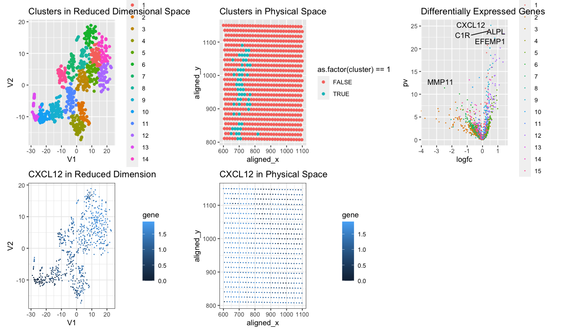
We are visualizing clusters in reduced dimensional space and identified cell cluster 1. We found this cell cluster to have several upregulated genes, including CXCL12, which plays a role in many diverse cellular functions, including embryogenesis, tissue homeostasis, and more. This cell cluster is clustered together in physical space as well. https://www.ncbi.nlm.nih.gov/gene/20315#:~:text=Cxcl12%20is%20an%20attractant%20for,of%20CD34%2B%20cells%20in%20microcirculation
library(Rtsne)
data<-read.csv(here("eevee.csv.gz"), row.names = 1)
pos<-data[,2:3]

gexp<-data[,4:ncol(data)]
gexp <- gexp[, colSums(gexp) > 1000]
gexp <- log10(gexp/rowSums(gexp) * mean(rowSums(gexp))+1)
reduced_data <- Rtsne(as.matrix(gexp), dims = 2)  # t-SNE
cluster_labels <- kmeans(reduced_data$Y, centers = 15)$cluster

# Combine cluster labels with original data
data_with_clusters <- data.frame(cbind(reduced_data$Y, cluster = as.factor(cluster_labels)))
cluster_data <- data_with_clusters[data_with_clusters$cluster == 1, ]
plot1 <- ggplot(data_with_clusters, aes(x = V1, y = V2, col = as.factor(cluster)),size=0.01) +
  geom_point() +
  ggtitle("Clusters in Reduced Dimensional Space (t-SNE)")+scale_colour_hue()
plot1

df<-data.frame(pos, data_with_clusters)
cluster_data <- df[df$cluster == 1, ]
plot2 <- ggplot(df, aes(x = aligned_x, y = aligned_y, col = as.factor(cluster)==1)) +
  geom_point() +
  ggtitle("Clusters in Physical Space")
plot2

head(cluster_data)
df2<-data.frame(pos, gexp, data_with_clusters)
cluster_data <- df2[df2$cluster == 1, ]

results <- sapply(colnames(gexp), function(g) {
  wilcox.test(gexp[cluster_labels == 1, g],
              gexp[cluster_labels != 1, g],
              gexp = "greater")$p.val
})
head(sort(results, decreasing=FALSE))

pv <- sapply(colnames(gexp), function(i) {
  #print(i) ## print out gene name
  wilcox.test(gexp[cluster_labels == 1, i], gexp[cluster_labels != 1, i])$p.val
})
logfc <- sapply(colnames(gexp), function(i) {
  #print(i) ## print out gene name
  log2(mean(gexp[cluster_labels == 1, i])/mean(gexp[cluster_labels != 1, i]))
})

df <- data.frame(pv=-log10(pv), logfc)
ggplot(df) + geom_point(aes(x = logfc, y = pv))
# challenge: label the extreme points (reccomend: ggrepel)
library(ggrepel)
geneclusters <- as.factor(kmeans(t(gexp), centers=15)$cluster)
df <- data.frame(pv=-log10(pv), logfc, geneclusters=geneclusters)
gg<-ggplot(df) + geom_point(aes(x = logfc, y = pv, col=geneclusters),size=0.01)

#gg + geom_text_repel(data = subset(df, pv > quantile(pv, 0.95) | logfc > quantile(logfc, 0.95)),
#                     aes(label = rownames(subset(df, pv > quantile(pv, 0.95) | logfc > quantile(logfc, 0.95)))))
extreme_points <- subset(df, pv > quantile(pv, 0.95) | logfc > quantile(logfc, 0.95))

# Label extreme points using ggrepel
plot3<-gg + geom_text_repel(data = extreme_points, aes(label = rownames(extreme_points), x = logfc, y = pv))+ggtitle("Differentially Expressed Genes")


plot4<-ggplot(data.frame(df2, gene = gexp[, 'CXCL12'])) +
  geom_point(aes(x = V1, y = V2, col=gene), size=.01) +
  theme_bw()+ggtitle("CXCL12 in Reduced Dimension")


plot5<-ggplot(data.frame(df2, gene = gexp[, 'CXCL12'])) +
  geom_point(aes(x = aligned_x, y = aligned_y, col=gene), size=.01) +
  theme_bw()+ggtitle("CXCL12 in Physical Space")
plot5
library(patchwork)
plot1+plot2+plot3+plot4+plot5