Differential Expression of APOD Gene in Barcode Data

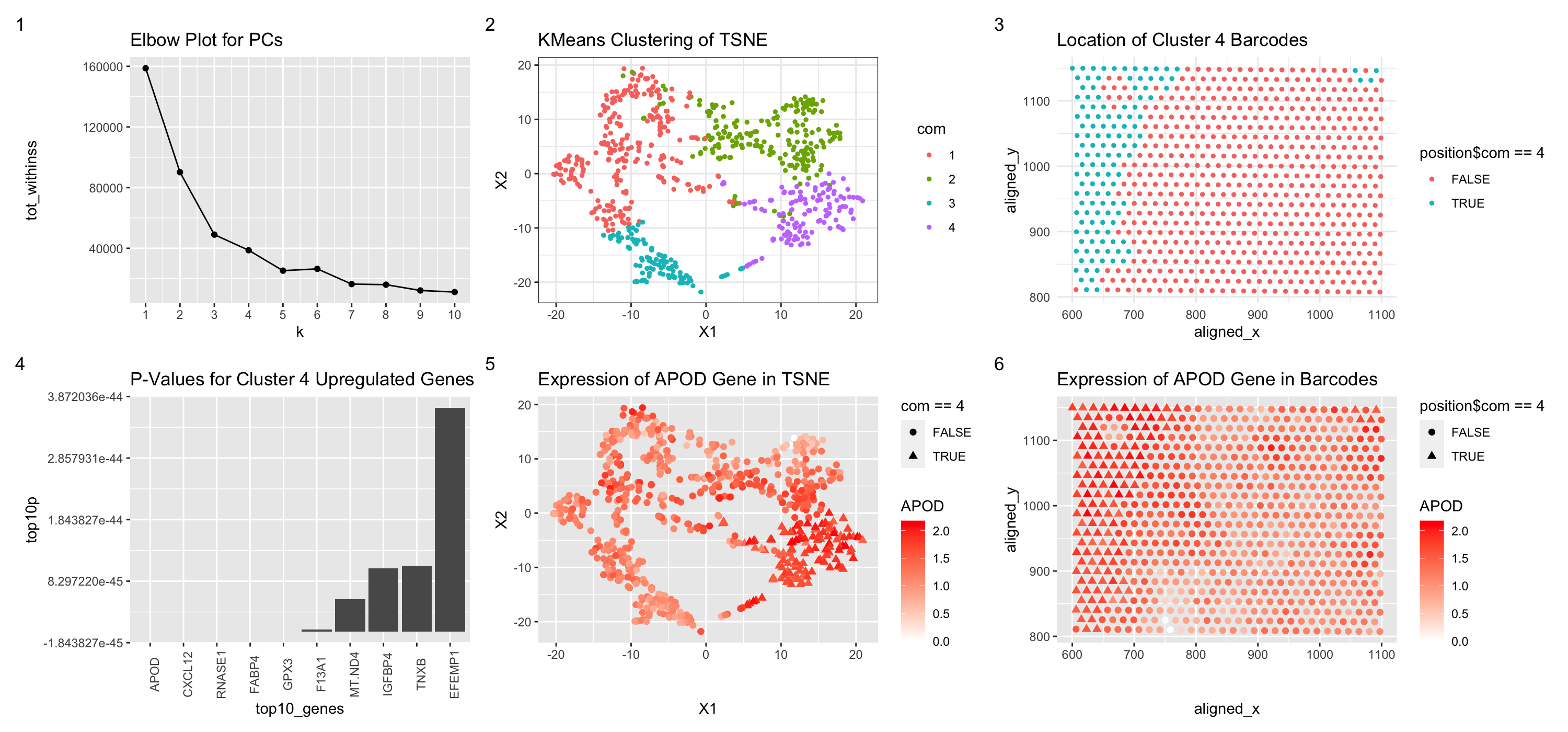
Figure Description
Figure 1 shows an elbow plot using points to display the withiness based on the k value. Figure 2 shows the 4 clusters created via kmeans clustering of the tsne plot of barcode data, with each point representing the values in this non-dimensional space based on gene expression. Color hue is used to represent the different clusters. Figure 3 shows the location of the cluster 4 barcodes in physical space, with color hue used to show whether the barcode is or isn’t a part of cluster 4. Figure 4 shows the p values from a greater-than t test for the differentially upregulated genes in cluster 4, each bar area representing the p-value. Figure 5 shows expression of the APOD gene in the tsne space, with shape of the points used to represent whether the barcode is a part of cluster 4 and color hue showing expression of the APOD gene. Figure 6 shows expression of the APOD gene in the physical barcode space, with hue used to represent expression and shape of the points used to represent whether the barcode is a part of cluster 4. Based on the p-values for a greater-than t test performed to compare the genes expressed in cluster 4 barcodes versus all other barcodes, genes such as CXCL12 and FABP4 are fare more common. This means we can assume that the cells in the cluster 4 barcodes more heavily express CXCL12 and FABP4. Visualization of expression of APOD further shows that cluster 4 is differentially displayed on the tsne plot. Further examination of two of the most highly upregulated genes, CXCL12 and FABP4, elucidates the possibility that cluster 4 barcodes are correlated with adipocytes. Adipocytes are found in connective tissue and often help with storage of energy (https://www.umassmed.edu/guertinlab/research/adipocytes/). CXCL12 is highly upregulated in adipocytes (https://www.proteinatlas.org/ENSG00000107562-CXCL12) and so is FABP4 (https://www.ncbi.nlm.nih.gov/pmc/articles/PMC4315049/). Furthermore, the highly upregulated gene of GPX3 is also often found in kidney cells, and thus the cluster 4 barcode cells may be adipocytes found near the visceral fat of the kidney.
data <- read.csv('~/OneDrive/Documents/School/Johns Hopkins/Spring 2024/eevee.csv.gz', row.names=1)
data[1:5,1:5]
pos <- data[,2:3]
gexp <- data[, 4:ncol(data)]

topgene <- names(sort(apply(gexp, 2, var), decreasing=TRUE)[1:1000])
gexp <- gexpfilter <- gexp[,topgene]

gexpnorm <- log10(gexp/rowSums(gexp) * mean(rowSums(gexp))+1)

pcs <- prcomp(gexpnorm)

# tsne
library(Rtsne)
emb <- Rtsne(pcs$x[,1:20])$Y # faster than tSNE on genes

library(purrr)

tot_withinss <- map_dbl(1:10,  function(k){
  model <- kmeans(x = emb, centers = k)
  model$tot.withinss
})
# Generate a data frame containing both k and tot_withinss
elbow_df <- data.frame(
  k = 1:10,
  tot_withinss = tot_withinss
)

library(ggplot2)
# Plot the elbow plot -> chose k = 4 https://www.r-bloggers.com/2020/05/how-to-determine-the-number-of-clusters-for-k-means-in-r/
elbow <- ggplot(elbow_df, aes(x = k, y = tot_withinss)) +
  geom_line() + geom_point()+
  scale_x_continuous(breaks = 1:10)

com <- as.factor(kmeans(gexpnorm, centers=4)$cluster)

#plot tsne with clusters
p1 <- ggplot(data.frame(emb, com)) +
  geom_point(aes(x = X1, y = X2, col=com), size=1) +
  theme_bw()

#plot location of clusters
position <- data.frame(pos, com)

physical <- ggplot(position) +
  geom_point(aes(x = aligned_x,
                 y=aligned_y,
                 col= position$com == 4),
             size=1) +
  theme_minimal()

#finding differentially expressed genes
gexpnorm$cluster <- com

results <- sapply(colnames(gexp), function(g) {
  t.test(gexpnorm[com == 4, g],
         gexpnorm[com != 4, g],
         alternative = "greater")$p.val
})
results

# find p values https://r-graph-gallery.com/218-basic-barplots-with-ggplot2.html
top10p <- sort(results, decreasing = FALSE)[1:10]

top10p

top10genes <- rownames(data.frame(top10p))

genes <- data.frame(top10p, top10genes)

#https://guslipkin.medium.com/reordering-bar-and-column-charts-with-ggplot2-in-r-435fad1c643e
#plot p values of top 10 upregulated genes
top10_genes <- reorder(top10genes, top10p)

p_values <- ggplot(genes, aes(x= top10_genes, y = top10p)) + geom_bar(stat='identity')

c4genes <- data.frame(gexpnorm[com == 4,][, top10genes])

nonc4genes <- data.frame(gexpnorm[com != 4,][, top10genes])

#https://www.geeksforgeeks.org/how-to-find-mean-of-dataframe-column-in-r/
#cluster 4 gene expressions
avg <- sapply(1:10, function(g) {
  mean(c4genes[, g])
})

#non cluster 4 gene expressions
nonavg <- sapply(1:10, function(g) {
  mean(nonc4genes[, g])
})

# https://www.tutorialspoint.com/how-to-create-a-replicated-list-of-a-list-in-r#:~:text=The%20replication%20of%20list%20of,(x)%2C5).
# https://www.digitalocean.com/community/tutorials/r-melt-and-cast-function

df1 <- data.frame(Cluster_4 = avg, Cluster_1to3 = nonavg)

df1 <- as.data.frame(melt(df1))
df1_new <- data.frame(df1, rep(colnames(c4genes), 2))
colnames(df1_new) <- c("Cluster", "Expression", "Gene")

# plot to display upregulated genes
upreg_genes <- ggplot(df1_new, aes(x = Gene, y = Cluster, fill = Expression)) +
  geom_tile() + scale_fill_gradient(low="white", high="red")

#choose gene APOD
apod_tsne <- ggplot(data.frame(emb, com, gexpnorm['APOD'])) +
  geom_point(aes(x = X1, y = X2, col = APOD, shape = com == 4), size=2) +
  scale_color_gradient(low="white", high="red")

apod_physical <- ggplot(data.frame(position, gexpnorm['APOD'])) +
  geom_point(aes(x = aligned_x, y=aligned_y, col= APOD, shape = position$com == 4),
             size=2) + scale_color_gradient(low="white", high="red")

# https://patchwork.data-imaginist.com/articles/guides/annotation.html
library(patchwork)

# https://www.datanovia.com/en/blog/ggplot-axis-ticks-set-and-rotate-text-labels/#:~:text=geom_boxplot()%20p-,Change%20axis%20tick%20mark%20labels,to%20rotate%20the%20tick%20text.
elbow <- elbow + ggtitle("Elbow Plot for PCs")
p1 <- p1 + ggtitle("KMeans Clustering of TSNE")
physical <- physical + ggtitle("Location of Cluster 4 Barcodes")
p_values <- p_values + ggtitle("P-Values for Cluster 4 Upregulated Genes") + theme(axis.text.x = element_text(angle = 90))
apod_tsne <- apod_tsne + ggtitle("Expression of APOD Gene in TSNE")
apod_physical <- apod_physical + ggtitle("Expression of APOD Gene in Barcodes")

elbow + p1 + physical + p_values + apod_tsne + apod_physical + plot_annotation(tag_levels = '1')