Interpreting cell cluster through dimensionality reduction and differential gene expression analysis

Things to know about my visualization

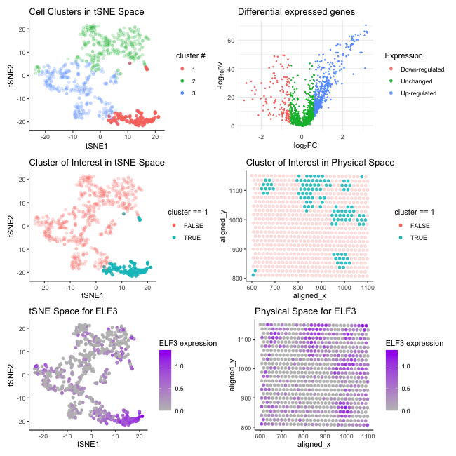
The visualization aims to provide evidence for characterizing a specific cluster of cells and understanding its gene expression profile. For data pre-processing, I first performed PCA on the normalized log-transformed gene expression data across the cell profile and then applied tSNE on the first 20 PCs generated from the previous linear dimensionality reduction step. Next, I performed K-means clustering to group the cells into 3 clusters by choosing the optimal value of K = 3 using the elbow method. Here’s a description of each panel:

1. Cell Clusters in t-SNE Space: This panel displays a t-SNE plot where cells (points) are grouped into three distinct clusters, using colors to endode different clusters.

2. Differential Expressed Genes: The volcano plot represents differential gene expression analysis results, with log2 fold-change on the x-axis and the negative log10 of the p-value on the y-axis. Points in this plot are color-coded to indicate upregulated, downregulated, and unchanged genes. The genes far from the center and high on the plot are considered significantly differentially expressed.

3. Cluster of Interest in t-SNE Space: This panel focuses on cluster 1, differentiating cells within the selected cluster from those outside it using color hues. Points represent cells are plotted in the tSNE space.

4. Cluster of Interest in Physical Space: This panel maps the same cluster of interest onto the physical coordinates of the tissue and use color hues to indicate the cluster.

5. t-SNE Space for ELF3: The expression level of the ELF3 gene is overlaid on the t-SNE plot. The color intensity indicates the level of ELF3 expression, with darker colors signifying higher expression levels.

6. Physical Space for ELF3: The final panel shows the spatial distribution of ELF3 expression across the physical coordinate of the tissue. Similary, the intensity of the color represents the gene’s expression level at each spot, indicating areas of higher and lower expression.

Which cell type does cluster 1 correspond to ?

My hypothesis is cluster 1 matches the profile with epithelial cells. First, the t-SNE clustering plots show that the cells within the cluster 1 have a unique gene expression profile compared to other cells. This uniqueness could be characteristic of a specific cell type, supported by the tight clustering observed, which suggests a high degree of similarity within the cluster. Then, by performing differential gene expression analysis, I selected a highly upregulated gene ELF3 (p-value = 3.75e-56, log2 fold change = 2.29), located in the upper right area on the volcano plot, to futher characterize cell identity. Previous published literature suggests ELF3 strongly correlates with an epithelial phenotype across cancer cell lines. [1] [2] Comparing both the tSNS and physical space plots for ELF3 expression patterns with those for cluster 1, we observe that the ELF3 gene expression is mainly mapped to cluster 1 with a few to spots belonging to other clusters and ELF3 is highly expressed in cluster 1. The above evidence provide a compelling argument for identifying cluster I being assoaicted with epithelial cells. For futher invesitgation, more information on spatial distribution can be helpful. For instance, epithelial cells typically line surfaces or cavities in tissues. If the physical space visualization of Cluster 1 aligns with areas known to be epithelial in nature, this spatial information would further support my hypothesis.

Reference:

1. Subbalakshmi, A. R., Sahoo, S., Manjunatha, P., Goyal, S., Kasiviswanathan, V. A., Mahesh, Y., Ramu, S., McMullen, I., Somarelli, J. A., & Jolly, M. K. (2023). The ELF3 transcription factor is associated with an epithelial phenotype and represses epithelial-mesenchymal transition. Journal of biological engineering, 17(1), 17. https://doi.org/10.1186/s13036-023-00333-z

2. Enfield, K.S.S., Marshall, E.A., Anderson, C. et al. Epithelial tumor suppressor ELF3 is a lineage-specific amplified oncogene in lung adenocarcinoma. Nat Commun 10, 5438 (2019). https://doi.org/10.1038/s41467-019-13295-y

library(ggplot2)
library(Rtsne)
library(tidyverse)
library(RColorBrewer)
library(patchwork)

data <- read.csv('eevee.csv.gz', row.names = 1)
pos <- data[,2:3]
gexp <- data[,4 :ncol(data)]
rownames(pos)<- rownames(data)<-data$barcode

# normalize data
gexp <-gexp[,colSums(gexp)>1000]
totalgen_exp <- rowSums(gexp)
norm_gexp <- gexp/totalgen_exp * median(totalgen_exp)
norm_gexp <- log10(norm_gexp + 1)

set.seed(200)
# PCA
pcs <- prcomp(norm_gexp)
# tSNE on 20 pcs
tsne_genes_res <- Rtsne(pcs$x[,1:20], dims = 2, perplexity = 30)

# pick optimal k using elbow method
# ref: https://www.r-bloggers.com/2017/02/finding-optimal-number-of-clusters/
k.max <- 8
wss <- sapply(1:k.max, 
              function(k){kmeans(norm_gexp, k, nstart=50,iter.max = 15 )$tot.withinss})
# elbow plot
plot(1:k.max, wss,
     type="b", pch = 19, frame = FALSE, 
     xlab="Number of clusters K",
     ylab="Total within-clusters sum of squares")

# pick k=3
com <- as.factor(kmeans(norm_gexp, center=3)$cluster)
data <- data.frame(pos, tsne_genes_res$Y, cellType = com)


alpha <- ifelse(data$cellType ==1, 0.85, 0.2)
# Reduced dimensional space visualization of all 3 clusters
p <- ggplot(data) + 
  geom_point(aes(x = X1, y = X2, col=cellType), alpha = alpha) +
  labs(title = 'Cell Clusters in tSNE Space',
       x = 'tSNE1', y = 'tSNE2', col = "cluster #") +
  theme_bw() +
  theme_classic()

# Panel 1: Reduced dimensional space visualization of the cluster
p1 <- ggplot(data) +
  geom_point(aes(x = X1, y = X2, color = (cellType ==1)), alpha = alpha) +
  theme_bw() + 
  labs(title = "Cluster of Interest in tSNE Space",
       x = "tSNE1", y = "tSNE2", col = "cluster == 1") +
  theme_classic()


# Panel 2: Physical space visualization of the cluster
p2 <- ggplot(data) +
  geom_point(aes(x = aligned_x, y = aligned_y, color = (cellType ==1)), alpha = alpha) +
  theme_bw() + 
  labs(title = "Cluster of Interest in Physical Space",
       col = "cluster == 1") +
  theme_classic()


# differential expression analysis 
#p-value
pv <- sapply(colnames(norm_gexp), function(i){
  wilcox.test(group1 <- norm_gexp[com == 1, i], norm_gexp[com != 1,i])$p.val
})

# Adjust p-values using the Benjamini-Hochberg correction
pv <- p.adjust(pv, method = "BH")

# log2 fold change
logfc <- sapply(colnames(norm_gexp), function(i){
  log2(mean(norm_gexp[com == 1, i])/mean(norm_gexp[com != 1, i]))
})


# Panel 3: volcano plot for differentially expressed genes
# ref: https://samdsblog.netlify.app/post/visualizing-volcano-plots-in-r/
volc_df <- data.frame(pv, logfc)
volc_df <- volc_df %>% 
  mutate(
    Expression = case_when(logfc >= 0.6 & pv <= 0.05 ~ "Up-regulated",
                           logfc <= -0.6 & pv <= 0.05 ~ "Down-regulated",
                           TRUE ~ "Unchanged")
  )

p3 <- ggplot(volc_df , aes(logfc, -log(pv,10))) +
  geom_point(aes(color = Expression), size = 2/5, alpha = 0.85) +
  xlab(expression("log"[2]*"FC")) + 
  ylab(expression("-log"[10]*"pv")) +
  ggtitle("Differential expressed genes")+
  theme_bw() +
  theme_minimal() +
  guides(colour = guide_legend(override.aes = list(size=1.5))) 

# Differentially expressed gene: ELF3
deg_df <- cbind(data, elf3 = norm_gexp$ELF3)
# Panel 4: Visualization of one DEG in reduced dimensional space
p4 <- ggplot(deg_df) +
  geom_point(aes(x = X1, y = X2, color= elf3)) +
  scale_color_gradient(low="grey", high="purple")+
  labs(title = "tSNE Space for ELF3",
       x = "tSNE1", y = "tSNE2", col = "ELF3 expression") +
  theme_classic()

# Panel 5: Visualization of one DEG in physical space
p5 <- ggplot(deg_df) +
  geom_point(aes(x = aligned_x, y = aligned_y, color= elf3)) +
  scale_color_gradient(low="grey", high="purple")+
  labs(title = "Physical Space for ELF3",col = "ELF3 expression") +
  theme_classic()

png(file="hw4_plot.png",
    width=650, height=650)
(p | p3)/ (p1 | p2) / (p4 | p5) 
dev.off()