Analyzing for Breast Glandular Cells

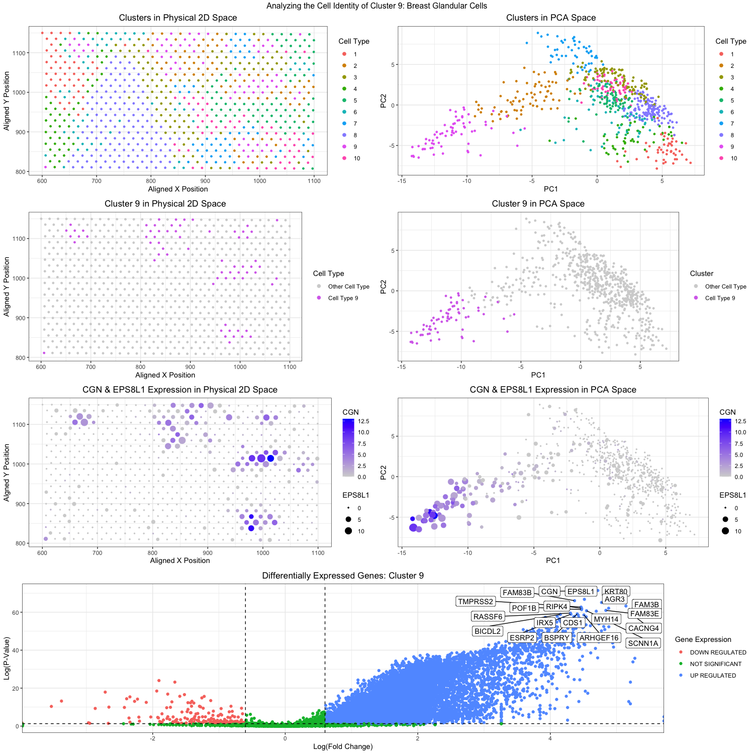
Figure Description:
Through k-means clustering and gene expression analysis, I wanted to identify a specific cell type in the breast cancer tissue in the eevee data set. To start off, I conducted a principal component analysis on the data. Then I determined that the optimal k would be 10 clusters, and hence I did the k-means analysis on the analyzed PCs. In the top right figure (plot2), you can see the clustering plotted with PC1 on the x-axis and PC2 on the y-axis, each color represents a different cluster, and each dot represents a spatial spot. Then I went back and plotted the clusters in the physical 2D space, again color coding the clusters in the top left figure (plot2). Based on these visualizations, I thought that cluster 9 was the most isolated and unique out of the ten clusters, with no overlap with other clusters. You can see this in the plots on the second row. The second left figure (plot3) shows the isolated cluster 9 in the 2D space, while the second right figure (plot4) shows the isolated cluster 9 in the PC space. From now on, all analysis was conducted with the spatial dots in cluster 9 only.
After normalization of the gene expressions, I used the sort function to order the gene expression in cluster 9 to find the highest/most upregulated genes expressed in those spatial dots. The top two genes I found to be up-regulated were CGN and EPS8L1. I was then able to visualize how upregulated the genes were in the cluster 9 dot. By encoding the levels of CGN expression with color saturation and the levels of EPS8L1 expression with size, I was able to visualize their expression in both the 2D space (plot5, third left figure) and the PC space (plot6, third right figure). These visualizations demonstrated that yes indeed, CGN and EPS8L1 were upregulated in the dots that overlap with the cluster 9 dots. CGN encodes for a protein called Cingulin, (in Latin it means “to form a belt around”). The protein localizes at the tight junctions of endothelial and epithelial cells to help in cell-cell adhesion and signaling (Guillemot et al, 2012). EPS8L1 on the other hand encodes for a protein that is related to epidermal growth factor receptor pathway substrate 8 (EPS8). There is not much known about the protein itself except that it is very multifunctional and also participates in cell-cell signaling pathways. However, its upregulation has been proven to help in metastasis and migration of ovarian cancer cells (Wang et al, 2022). Unfortunately, we cannot determine for sure what exact cell type cluster 9 is, we can at least say it is probably of epithelial origins and perhaps may be involved in the cancer that is present in this breast tissue sample. Lastly, I want to look at all the differentially expressed genes in cluster 9. A one-sided Wilcox test was done for each gene to determine if it was differentially expressed in the dots in cluster 9 or not. Visualization was done with color coding hues to represent if the genes were down-regulated, not significantly regulated, or upregulated in cluster 9. The results can be seen in the very bottom figure (plot7). Genes that have significant differential expression are also labeled in the figure and emphasized. Looking at some of these upregulated genes we can try to further our determination of the cell type. For one, FAM83B which seems also to be significantly upregulated. The upregulation of FAM83B is also associated with cancer metastasis in breast, lung and pancreatic cancers (Cirello et al, 2022). Another gene that is upregulated and associated with cancer is the IRX5 gene that is also shown in plot7. IRX5 encodes for Iroquois homeobox protein 5, which is a transcription factor that is essential in tissue differentiation and embryonic development. Its upregulation is very much indicative of cancer and it’s been shown that there is a correlation between IRX5 and BRCA1 (literally known as breast cancer type 1 susceptibility protein) which might indicate that the spots in cluster 9 might be cancer epithelial cells (Chen et al, 2023).
Links / Other References:
References: Guillemot, L., Schneider, Y., Brun, P., Castagliuolo, I., Pizzuti, D., Martines, D., Jond, L., Bongiovanni, M., & Citi, S. (2012). Cingulin is dispensable for epithelial barrier function and tight junction structure, and plays a role in the control of claudin-2 expression and response to duodenal mucosa injury. Journal of cell science, 125(Pt 21), 5005–5014. https://doi.org/10.1242/jcs.101261
Yuting Wang, Lei Zhang, Xianqiang Luo, et al. EPS8L1 promotes migration and metastasis of ovarian cancer by activating Rac1/MAPK signaling pathway via upregulating TIAM2. Authorea. December 16, 2022. DOI: 10.22541/au.167120661.17798120/v1
Cirello, V., Grassi, E.S., Pogliaghi, G. et al. FAM83B is involved in thyroid cancer cell differentiation and migration. Sci Rep 12, 8608 (2022). https://doi.org/10.1038/s41598-022-12553-2
Chen, J. K., Wiedemann, J., Nguyen, L., Lin, Z., Tahir, M., Hui, C. C., Plikus, M. V., & Andersen, B. (2023). IRX5 promotes DNA damage repair and activation of hair follicle stem cells. Stem cell reports, 18(5), 1227–1243. https://doi.org/10.1016/j.stemcr.2023.03.013
## Packages for graphing
library(ggplot2)
library(dplyr)
library(gridExtra)
library(ggrepel)

## Packages for determining optimal cluster number
library(factoextra)
library(NbClust)
library(cluster)

## Load the data
data <- read.csv('eevee.csv.gz', row.names = 1)

## Isolate columns of interest
pos <- data[,2:3]
gexp <- data[, 4:ncol(data)]

## Isolate cells that have gene Expression
good_cells <- rownames(gexp)[rowSums(gexp) > 0]
pos <- pos[good_cells,]
gexp <- gexp[good_cells,]

## Normalize the data
tot_gexp <- rowSums(gexp)
norm_gexp <- gexp/tot_gexp * median(tot_gexp)
log_norm_gexp <- log10(norm_gexp + 1)

## Run PCA on the data
pcs <- prcomp(log_norm_gexp)

## Determine optimal number of PCs to run for kMeans
plot(1:50, pcs$sdev[1:50], type = 'l')
plot(1:20, pcs$sdev[1:20], type = 'l')
plot(1:10, pcs$sdev[1:10], type = 'l')

## Appears that having 9 PCs is enough to account for most
## of the variance in the data.
optimal_pc_num <- 9

## Determine the optimal number of k's (centroids) for kMeans

## Gap Statistic
set.seed(123)
gap_stat <- clusGap(log_norm_gexp, FUNcluster = kmeans, K.max = 10, B = 50)
fviz_gap_stat(gap_stat)

## Identifying optimal number of k's
optimal_k <- 10

## Set seed for reproducibility
set.seed(1)

## Run kMeans
cluster_pcs <- kmeans(pcs$x[,1:optimal_pc_num], centers = optimal_k)
df_cluster <- data.frame(pos, cell_type = as.factor(cluster_pcs$cluster), gexp, pcs$x[,1:10])

## Visualizing cells in the 2D space
clusters_2D <- ggplot(data = df_cluster, aes(x = aligned_x, y = aligned_y, col = cell_type)) +
  geom_point(size = 1) +
  theme_bw() +
  theme(plot.title = element_text(hjust = 0.5)) +
  xlab("Aligned X Position") + ylab("Aligned Y Position") +
  guides(color = guide_legend(override.aes = list(size = 2))) +
  labs(title = 'Clusters in Physical 2D Space', col = "Cell Type")

clusters_2D

## Visualizing cells in the PCA space
clusters_PCA <- ggplot(data = df_cluster, aes(x = PC1, y = PC2, col = cell_type)) +
  geom_point(size = 1) +
  theme_bw() +
  theme(plot.title = element_text(hjust = 0.5)) +
  guides(color = guide_legend(override.aes = list(size = 2))) +
  labs(title = 'Clusters in PCA Space', col = "Cell Type")

clusters_PCA

## Picking a cluster (cluster 9)

## Visualizing Cluster 9 in Physical 2D Space
cluster9_2D <- ggplot(data = df_cluster, aes(x = aligned_x, y = aligned_y, col = cell_type == 9)) +
  geom_point(size = 1) +
  theme_bw() +
  theme(plot.title = element_text(hjust = 0.5)) +
  guides(color = guide_legend(override.aes = list(size = 2))) +
  labs(title = 'Cluster 9 in Physical 2D Space') +
  xlab("Aligned X Position") + ylab("Aligned Y Position") +
  scale_color_manual(name = 'Cell Type',
                     values = c('lightgrey', '#D772EC'),
                     labels = c('Other Cell Type', 'Cell Type 9'))

cluster9_2D

## Visualizing Cluster 9 in the PCA Space
cluster9_PCA <- ggplot(data = df_cluster, aes(x = PC1, y = PC2, col = cell_type == 9)) +
  geom_point(size = 1) +
  theme_bw() +
  theme(plot.title = element_text(hjust = 0.5)) +
  guides(color = guide_legend(override.aes = list(size = 2))) +
  labs(title = 'Cluster 9 in PCA Space') +
  scale_color_manual(name = 'Cluster',
                     values = c('lightgrey', '#D772EC'),
                     labels = c('Other Cell Type', 'Cell Type 9'))

cluster9_PCA

## Distinguishing between cells that are & are not within Cluster 9
cluster9 <- df_cluster[df_cluster$cell_type == 9, ]
not_cluster9 <- df_cluster[df_cluster$cell_type != 9, ]

## Identifying differentially expressed genes w/in Cluster 9 w/ Wilcox Rank Test
interest_genes <- sapply(colnames(gexp), function(g){
  wilcox.test(gexp[row.names(cluster9), g],
              gexp[row.names(not_cluster9), g])$p.value
})

## Calculating log(fold_change) for Cluster 9 --> to generate volcano plot
log_fc <- sapply(colnames(gexp), function(g) {
  log2( mean(gexp[row.names(cluster9), g])
        / mean(gexp[row.names(not_cluster9), g])) ## do ratio (log_2(A/B))
})

volcano <- data.frame(log_fc, log_p_val = -log10(interest_genes))
genes_upregulated <- sapply(colnames(gexp), function(g){
  wilcox.test(gexp[row.names(cluster9), g],
              gexp[row.names(not_cluster9), g],
              alternative = 'greater')$p.value
})

top_20_genes <- sort(genes_upregulated, decreasing = FALSE)[1:20]
top_20_genes

## For coloring in the points for volcano plot
volcano$diff_express <- "NOT SIGNIFICANT"
volcano$diff_express[volcano$log_fc > 0.6 & volcano$log_p_val > -log10(0.05)] <- "UP REGULATED"
volcano$diff_express[volcano$log_fc < -0.6 & volcano$log_p_val > -log10(0.05)] <- "DOWN REGULATED"

## Creating volcano plot to visualize upregulated genes in Cluster 9!
volcano_plot <- ggplot(volcano) +
  geom_point(aes(x = log_fc, y = log_p_val, col = diff_express)) +
  geom_vline(xintercept = c(-0.6, 0.6), linetype = 'dashed') +
  geom_hline(yintercept=-log10(0.05), linetype = 'dashed') +
  geom_label_repel(data= volcano[names(top_20_genes),],
                   aes(x = log_fc, y = log_p_val, label = names(top_20_genes)),
                   max.overlaps = 40) +
  theme_bw() +
  labs(title = 'Differentially Expressed Genes: Cluster 9',
       x = 'Log(Fold Change)', y = 'Log(P-Value)', col = "Gene Expression") +
  theme(plot.title = element_text(hjust = 0.5))

volcano_plot

## Plot the top 2 most significant genes (CGN, EPS8L1)

## Plotting in Physical 2D Space
gene_2d <- ggplot(data = data, aes(x = aligned_x, y = aligned_y, col = CGN, size = EPS8L1)) +
  geom_point() +
  theme_bw() +
  scale_color_gradient(low = 'lightgrey', high = 'blue') +
  scale_size(range = c(0.5, 5)) +
  labs(x = "Aligned X Position", y = "Algned Y Position", size = "EPS8L1", color = "CGN", title = "CGN & EPS8L1 Expression in Physical 2D Space") +
  theme(plot.title = element_text(hjust = 0.5))

gene_2d

## Plotting in PCA Space
gene_pca <- ggplot(data = df_cluster, aes(x = PC1, y = PC2, col = CGN, size = EPS8L1)) +
  geom_point() +
  theme_bw() +
  scale_color_gradient(low = 'lightgrey', high = 'blue') +
  scale_size(range = c(0.5, 5)) +
  labs(size = "EPS8L1", color = "CGN", title = "CGN & EPS8L1 Expression in PCA Space") +
  theme(plot.title = element_text(hjust = 0.5))

gene_pca

## Combining all the plots together
lay <- rbind(c(1,2),
             c(3,4),
             c(5,6),
             c(7,7))

grid.arrange(clusters_2D, clusters_PCA,
             cluster9_2D, cluster9_PCA,
             gene_2d, gene_pca,
             volcano_plot,
             layout_matrix = lay,
             top = "Analyzing the Cell Identity of Cluster 9: Breast Glandular Cells")

## References:
## (1) To determine the optimal number of clusters
## https://medium.com/@chyun55555/how-to-find-the-optimal-number-of-clusters-with-r-dbf84988388b
## (2) Graphing volcano plots
## https://biocorecrg.github.io/CRG_RIntroduction/volcano-plots.html