Expression of MMP7 in physical space and reduced dimensional space

Describe your figure briefly
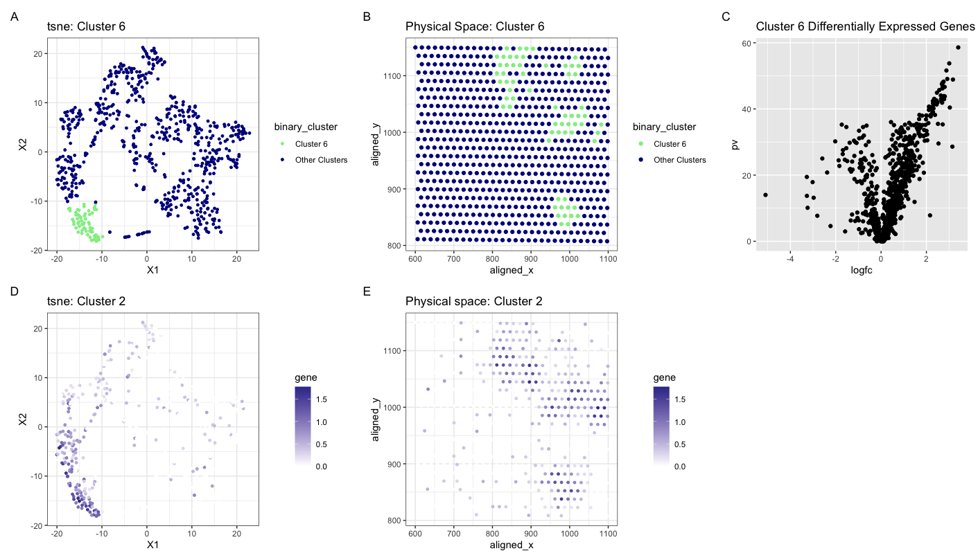
My plot visualizes the expression of MMP7 both in physical space in spacial barcode bead capture and in reduced dimensional space. The plots show cluster 6 highlighted in reduced dimensional space (tSNE) and physical space as my cluster of interest. They then show my gene of interest, MMP7 in physical and reduced dimensional space to compare where they lie in comparison to each other. From top to bottom and left to right are plots A, B, C, D, and E. (A) displays a tSNE mapping of how the cells are clustered with cluster 6 highlighted in light green. (B) maps cluster 6 into the physical space with aligned x and aligned y and shows the physical location in each bead. (C) is a volcano plot that displays differentially expressed genes in cluster 6. (D) shows a tSNE plot of specifically MMP7 in the clusters. And (E) shows the expression of MMP7 in physical space in each bead. For plots D and E, a darker blue color correlates with a higher expression of MMP7. MMP7 is involved in producing proteins that breakdown the extracellular matrix and play a big role in cancer metastasis (1). In fact, previous studies have concluded that MMP7 expression serves as a biomarker for breast cancer metastasis particularly to the lungs and brain (2). Knowing that the eevee and pikachu datasets are both obtained from breast cancer tissue, I believe that my identification of MMP7 is correct. In addition, MMP7 serves as a mediator of lung inflammation and repair after damage (3), which leads me to think that the cluster I have identified are lung cells in which breast cancer tumor has metastatisized to.
- https://www.ncbi.nlm.nih.gov/gene/4316
- https://www.ncbi.nlm.nih.gov/pmc/articles/PMC4716673/#:~:text=Analysis%20of%20publically%20available%20datasets,lines%20and%20patient%20tumor%20samples
- https://www.ncbi.nlm.nih.gov/pmc/articles/PMC3604090/
Please share the code you used to reproduce this data visualization.
```{r} #install.packages(‘Rtsne’) #install.packages(‘ggplot2’)
library(Rtsne) library(ggplot2) library(patchwork)
data <- read.csv(‘/Users/conniechen/Documents/Genomic Data Visualization 2024/GDV HW/eevee.csv.gz’, row.names = 1) dim(data)
pos <- data[, 2:3] gexp <- data[, 4:ncol(data)]
Limit the number of genes
topgene <- names(sort(apply(gexp, 2, var), decreasing=TRUE)[1:1000]) gexpfilter <- gexp[,topgene] dim(gexpfilter)
Normalization
gexpnorm <- log10(gexpfilter/rowSums(gexpfilter) * mean(rowSums(gexpfilter))+1)
PCA
pcs <- prcomp(gexpnorm) dim(pcs$x) #plot(pcs$sdev[1:30])
tsne
emb <- Rtsne(pcs$x[,1:15])$Y
Kmeans clustering and tsne plotting
com <- as.factor(kmeans(gexpnorm, centers=10)$cluster)
Changing cluster colors
help from chatgpt
binary_cluster <- ifelse(com == 6, “Cluster 6”, “Other Clusters”) binary_cluster <- as.factor(binary_cluster)
plotting tsne cluster 2
p1 <- ggplot(data.frame(emb, binary_cluster), aes(x = X1, y = X2, col=binary_cluster)) + geom_point(size=1) + theme_bw() + ggtitle(‘tsne: Cluster 6’) + scale_color_manual(values = c(“Cluster 6” = “light green”, “Other Clusters” = “dark blue”))
plotting physical space cluster 6
p2 <- ggplot(data) + geom_point(aes(x = aligned_x, y = aligned_y, col = binary_cluster)) + theme_bw() + ggtitle(‘Physical Space: Cluster 6’) + scale_color_manual(values = c(“Cluster 6” = “light green”, “Other Clusters” = “dark blue”))
pv versus log fc
pv <- sapply(colnames(gexpnorm), function(i) { #print(i) ## print out gene name wilcox.test(gexpnorm[com == 6, i], gexpnorm[com != 6, i])$p.val }) logfc <- sapply(colnames(gexpnorm), function(i) { #print(i) ## print out gene name log2(mean(gexpnorm[com == 6, i])/mean(gexpnorm[com != 6, i])) })
df <- data.frame(pv=-log10(pv), logfc) p3 <- ggplot(df) + geom_point(aes(x = logfc, y = pv)) + ggtitle(‘Cluster 6 Differentially Expressed Genes’)
p1 + p2 + p3
tsne for gene MMP7
geneclusters <- as.factor(kmeans(t(gexpnorm), centers=10)$cluster) head(geneclusters[geneclusters == 6])
df2 <- data.frame(emb, gene=gexpnorm[, ‘MMP7’]) df3 <- data.frame(pos, gene = gexpnorm[, ‘MMP7’]) p4 <- ggplot(df2) + geom_point(aes(x = X1, y = X2, col=gene), size=1) + theme_bw() + ggtitle(‘tsne: Cluster 2’) + scale_color_gradient2(high = scales::muted(“blue”), mid = ‘white’, low = scales::muted(“red”))
Cluster 2 in physical space
p5 <- ggplot(df3) + geom_point(aes(x = aligned_x, y = aligned_y, col=gene), size=1) + theme_bw() + ggtitle(‘Physical space: Cluster 2’) + scale_color_gradient2(high = scales::muted(“blue”), mid = ‘white’, low = scales::muted(“red”))
p1 + p2 + p3 + p4 + p5