Cell Cluster Identification and Validation in Breast Tumor Tissue
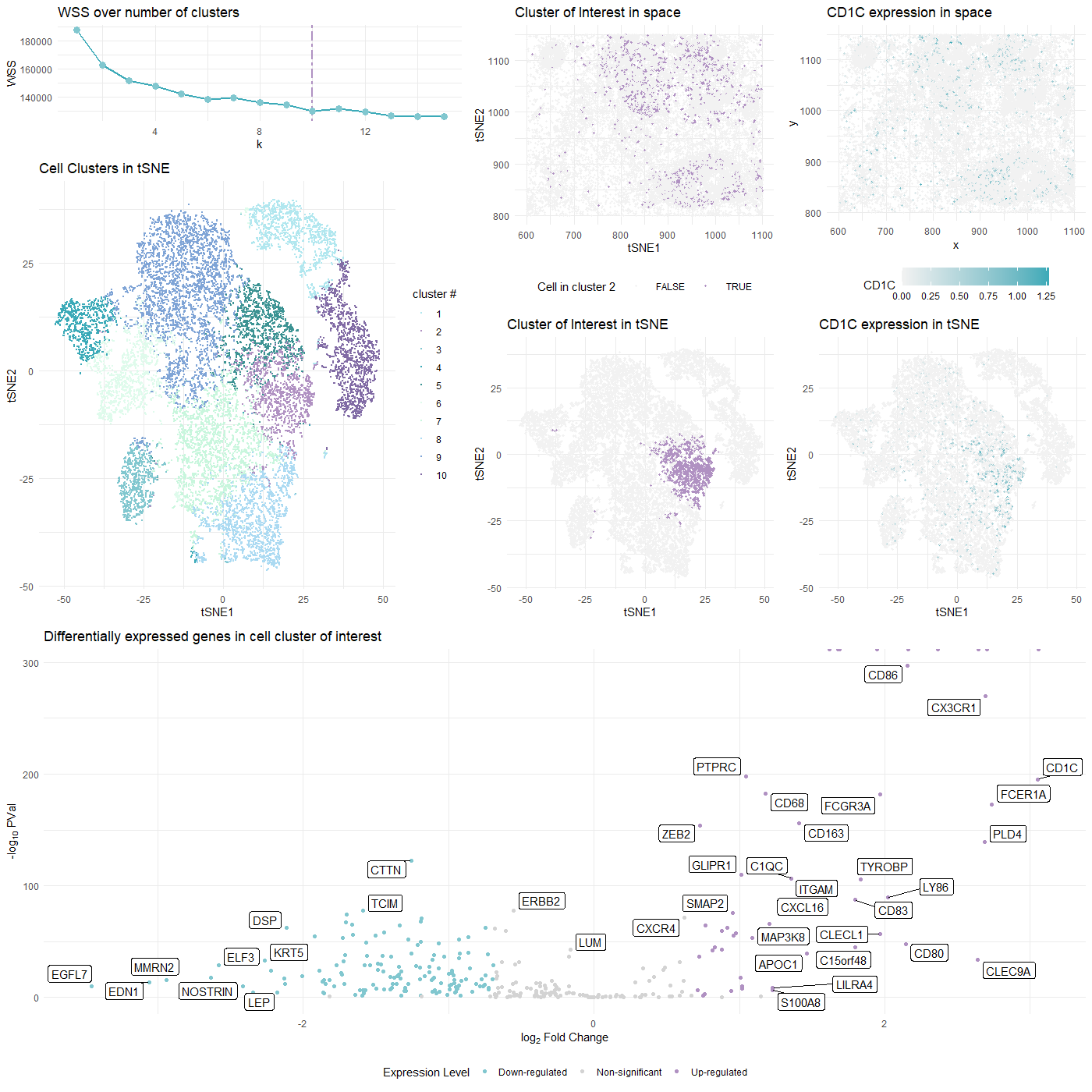
### Plot Description This visualization presents differential gene expression to validate cell type identification by k-means on 2D tSNE space.
-
The spatial-transcriptomics data on breast tumor tissue is preprocessed by removing cells with total gene counts below 10, normalized by total gene counts, and log-scaled.
-
The 10 cell clusters (see WSS curve for choice of k) are encoded by different colors in tSNE space to show the perfomance of k-means clustering. The 10 clusters also roughly matches number of potential cell types within the tissue.
-
Epithelial Cells, Fibroblasts, Adipocytes, Macrophages, Dendritic Cells, NK Cells (Natural Killer Cells), T Cells (CD4+ and CD8+), γδ T Cells, Mast Cells, Cancer Stem Cells (CSCs)
- A cluster is randomly selected as cluster of interest and identified in both tSNE and physical space with the same color used in the 10-cluster plot.
-
The most differentially expressed genes are computed in the selected cluster through two-sided Wilcox test, and demonstrated on the volcano plot.
-
The most up-regulated (and cancer-related) CD1c gene’s distribution is plotted in both tSNE and physical space
Cluster of Interest
The selected cluster of insterest (cluster 2) is highly possible to be CD1c+CD14+ dendritic cells (DC), characterized by the marker gene CLEC9A, as indicated as highly-expressed within the cluster on the volcano plot.
Expression of human CLEC9A is highly restricted in peripheral blood, being detected only on BDCA3+ dendritic cells and on a small subsetof CD14+CD16- monocytes [1].
In general, the differentially expressed genes are also consistent with the claim that the cluster of interest corresponds to immune cells within tumor tissue.
- Up-regulated CD1C
While CD1c is thought to specifically identify this subset of human cDCs, we show here that also classical and intermediate monocytes express CD1c. Accordingly, the commercial CD1c (BDCA-1)+ Dendritic Cell Isolation Kit isolates two distinct cell populations from blood: CD1c+CD14− cDCs and CD1c+CD14+ monocytes [2].
For example, studies of plasmacytoid pre-DCs (pDCs) and the cDC1 and cDC2 subsets of conventional DCs (CD141+ DCs and CD1c+ DCs, respectively) from human blood and tonsils have revealed that pDCs cluster first by ontogeny independently of their tissue of origin [3].
- Down-regulated EGFL7 EGFL7 alters cellular adhesion to the ECM and migratory behavior of tumor and immuno-cancer cells contributing to tumor metastasis [4].
- Down-regulated MMRN2 The down-modulation of MMRN2 occurs also in the context of tumor-associated angiogenesis. Immunofluorescence performed on tumor sections indicate a broad co-localization of MMP-9 and MMRN2, suggesting that the molecule may be extensively remodeled during tumor angiogenesis [5].
The possibility of the cluster being undifferentiated monocytes[2], as supported by the literature above, is eliminated by the follwing reasonings:
- Monocytes circulates in the bloodstream, while DCs are more commonly fixed to a specific tissue.
- DC-related genes are generally up-regulated in the cluster of interest, though there is no support for the specificity of the genes.
- The distribution in physical and tSNE spaces of CD1c, which is more commonly a DC identifier, are substantially aligned with the cluster’s distribution.
References
[1] Huysamen C, Willment JA, Dennehy KM, Brown GD. CLEC9A is a novel activation C-type lectin-like receptor expressed on BDCA3+ dendritic cells and a subset of monocytes. J Biol Chem. 2008 Jun 13;283(24):16693-701. doi: 10.1074/jbc.M709923200. Epub 2008 Apr 11. PMID: 18408006; PMCID: PMC2562446.
[2] Schrøder M, Melum GR, Landsverk OJ, Bujko A, Yaqub S, Gran E, Aamodt H, Bækkevold ES, Jahnsen FL, Richter L. CD1c-Expression by Monocytes - Implications for the Use of Commercial CD1c+ Dendritic Cell Isolation Kits. PLoS One. 2016 Jun 16;11(6):e0157387. doi: 10.1371/journal.pone.0157387. PMID: 27311059; PMCID: PMC4911075.
[3] Michea, P., Noël, F., Zakine, E. et al. Adjustment of dendritic cells to the breast-cancer microenvironment is subset specific. Nat Immunol 19, 885–897 (2018). https://doi.org/10.1038/s41590-018-0145-8
[4] Heissig B, Salama Y, Takahashi S, Okumura K, Hattori K. The Multifaceted Roles of EGFL7 in Cancer and Drug Resistance. Cancers (Basel). 2021 Mar 1;13(5):1014. doi: 10.3390/cancers13051014. PMID: 33804387; PMCID: PMC7957479.
[5] Andreuzzi E, Colladel R, Pellicani R, Tarticchio G, Cannizzaro R, Spessotto P, Bussolati B, Brossa A, De Paoli P, Canzonieri V, Iozzo RV, Colombatti A, Mongiat M. The angiostatic molecule Multimerin 2 is processed by MMP-9 to allow sprouting angiogenesis. Matrix Biol. 2017 Dec;64:40-53. doi: 10.1016/j.matbio.2017.04.002. Epub 2017 Apr 21. PMID: 28435016.
Source Code
## load dataset
data <- read.csv('C:/Users/ivych/OneDrive - Johns Hopkins/Classes/Data Visualization/pikachu.csv.gz', row.names = 1)

# install.packages("Rtsne")
## import libraries
library(ggplot2)
library(gridExtra)
library(Rtsne)

## set theme
plot_theme <- theme_bw() +
  theme(text = element_text(size = 10), legend.key.size = unit(0.5, 'cm'))
#ref: https://www.color-hex.com/color-palette/1022322
xiao_plt <- c("#b1e7ef",
              "#B091C2",
              "#81c7cf",
              "#3BAAB8",
              "#3c9393",
              "#DFFBEC",
              "#C8F6DD",
              "#abdaf2",
              "#7fa4d6",
              "#816BA5")

## data selection
pos <- data[,4:5]
gexp <- data[,6:ncol(data)]
good.cells <-rownames(gexp)[rowSums(gexp) > 10]
pos <- pos[good.cells,]
gexp <- gexp[good.cells,]

## normalization
gexp_norm <- gexp*median(rowSums(gexp))/rowSums(gexp)
gexp_log <- log10(gexp_norm+1)
mat <- unique(gexp_log)

#scree plot for pcs
x <- 1:15
pcs <- prcomp(mat)
par(mfrow=c(1,1))
data_scree <- data.frame(x = x, std = pcs$sdev[1:15])
ggplot(data_scree, aes(x, std)) +
  geom_line(color = xiao_plt[4], size = 1) +
  geom_point(color = xiao_plt[3], size = 3) +
  labs(title = "Scree plot", x = "Number of PCs", y = "STD") +
  theme_minimal()
#pcs = 8

#pcs and tsne
pcs_result <- pcs$x[,1:8]
tsne_result <- Rtsne::Rtsne(pcs_result)

## elbow method for clustering
wss <- numeric(15)
for (i in 1:15) {
  wss[i] <- sum(kmeans(mat, centers = i)$withinss)
}
data_elbow <- data.frame(x = x, wss = wss)
p_elbow <- ggplot(data_elbow, aes(x, wss)) +
  geom_segment(col = xiao_plt[2], size=1, linetype = 'twodash',
               aes(x = 10, y = Inf, xend = 10, yend = -Inf)) +
  geom_line(color = xiao_plt[4], size = 1) +
  geom_point(color = xiao_plt[3], size = 3) +
  labs(title = "WSS over number of clusters", x = "k", y = "WSS") +
  theme_minimal()

## K-means
#k = 10 seems to give the optimal result
com = kmeans(mat, center  = 10)
df <- data.frame(pos, tsne_result$Y, celltype=as.factor(com$cluster))
head(df)
p_k <- ggplot(df) +
  geom_point(size = 0.4,aes(x = X1, y = X2, col=celltype)) +
  labs(title = 'Cell Clusters in tSNE',
       x = 'tSNE1', y = 'tSNE2', col = "cluster #") +
  theme_minimal() + # theme(legend.position = "none") +
  scale_colour_manual(values = xiao_plt)

# pick cluster of interest
coi <- 2

#cluster of interest in the tsne space
p_c1 <- ggplot(df) +
  geom_point(size = 0.7,aes(x = X1, y = X2, col=(celltype==coi))) +
  labs(title = 'Cluster of Interest in tSNE',
       x = 'tSNE1', y = 'tSNE2',col="in cluster 2") +
  theme_minimal() + theme(legend.position = "none") +
  scale_colour_manual(values = c("grey95",xiao_plt[coi]))

#cluster of interest in the physical space
p_c2 <- ggplot(df) +
  geom_point(size = 0.7, aes(x = aligned_x, y = aligned_y, col=(celltype==coi))) +
  labs(title = 'Cluster of Interest in space',
       x = 'tSNE1', y = 'tSNE2',col="Cell in cluster 2") +
  theme_minimal() + theme(legend.position = "bottom", legend.key.size = unit(1, "cm")) +
  scale_colour_manual(values = c("grey95",xiao_plt[coi]))


## Double-sided wilcox test to identify differential expression
cluster.oi<- names(which(com$cluster == coi))
cluster.ot <- names(which(com$cluster != coi))

#differential genes
genes <- colnames(mat)
pvs <- sapply(genes, function(g) {
  oi <- mat[cluster.oi, g]
  ot <- mat[cluster.ot, g]
  wilcox.test(oi, ot, alternative="two.sided")$p.val})

names(which(pvs < 1e-100))
head(sort(pvs), n=15)

#fold change
log2fc <- sapply(genes, function(g) {
  oi <- mat[cluster.oi, g]
  ot <- mat[cluster.ot, g]
  log2(mean(oi)/mean(ot))})

#volcano plot
df_volcano <- data.frame(pvs, log2fc)
exp_sig <- apply(df_volcano, 1, function(g) {
  if (g[2] >= log(2) & g[1] <= 0.05) {out = "Up-regulated"}
  else if (g[2] <= -log(2) & g[1] <= 0.05) {out = "Down-regulated"}
  else {out = "Non-significant"}
  out})
data_deg <- cbind(df_volcano, exp_sig)

#install.packages("ggrepel")

p_volc <- ggplot(data_deg, aes(y=-log10(pvs), x=log2fc)) +
  scale_color_manual(values = c(xiao_plt[3], "lightgray", xiao_plt[2])) +
  geom_point(aes(col = exp_sig)) +
  ggrepel::geom_label_repel(label=rownames(data_deg)) +
  xlab(expression("log"[2]*" Fold Change")) +
  ylab(expression("-log"[10]*" PVal")) +
  theme_minimal()+
  theme(legend.position = 'bottom') +
  labs(title = 'Differentially expressed genes in cell cluster of interest',
       col = "Expression Level")

# Visualize CD1C
# https://bmccancer.biomedcentral.com/articles/10.1186/s12885-023-10558-2#:~:text=CD1C%20is%20an%20important%20part%20of%20the%20TME,and%20a%20new%20treatment%20target%20for%20breast%20cancer.

df_cd1c <- cbind(df,CD1C = mat$CD1C)

p_cd1c1 <-ggplot(df_cd1c) +
  geom_point(size = 0.7,aes(x = aligned_x, y = aligned_y, col = CD1C)) +
  theme_minimal() + theme(legend.position="bottom", legend.key.width = unit(1, "cm")) +
  labs(title = 'CD1C expression in space',
       x = 'x', y = 'y') +
  scale_color_gradient(low = 'grey95', high=xiao_plt[4])

p_cd1c2 <- ggplot(df_cd1c) +
  geom_point(size = 0.7,aes(x = X1, y = X2, col = CD1C)) +
  theme_minimal()+ theme(legend.position="none", legend.key.size = unit(0.2, "cm")) +
  labs(title = 'CD1C expression in tSNE',
       x = 'tSNE1', y = 'tSNE2') +
  scale_color_gradient(low = 'grey95', high=xiao_plt[4])


#plot panel arrangement
layout <- rbind(c(1,1,1,3,3,4,4),
                c(2,2,2,3,3,4,4),
                c(2,2,2,5,5,6,6),
                c(2,2,2,5,5,6,6),
                c(7,7,7,7,7,7,7),
                c(7,7,7,7,7,7,7),
                c(7,7,7,7,7,7,7))
grid.arrange(p_elbow,p_k,
             p_c2,p_cd1c1,
             p_c1,p_cd1c2,
             p_volc,
             layout_matrix = layout)