Identifying Glandular Cells and Adipocytes in Breast Tissue

Describe your figure briefly so we know what you are depicting (you no longer need to use precise data visualization terms as you have been doing). Write a description to convince me that your cluster interpretation is correct. Your description may reference papers and content that allowed you to interpret your cell cluster as a particular cell-type. You must provide attribution to external resources referenced. Links are fine; formatted references are not required. You must include the entire code you used to generate the figure so that it can be reproduced.

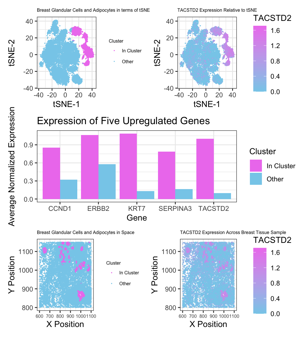
I chose to cluster my data around 7 centers after comparing total withiness for different k values. I selected the cluster which I believe to be breast glandular cells and adipocytes. I am visualizing my cluster in reduced dimensional space with tSNE in panel A and spatially in panel B, with my cluster of interest being purple against the black cells of other clusters. In panel C, I am comparing normalized gene expression of five upregulated genes in my cluster and the other cells. I selected these genes because they had the highest levels of expression in my cluster of all of the genes with p-values equal to zero based on a Wilcox test. In panels D and E, I am visualizing expression of TACSTD2, one of those genes, in terms of tSNE and spatial location respectively.

I first looked at the Protein Atlas profiles for the five genes with the highest average normalized expression (KRT7, TACSTD2, ERBB2, SERPINA3, and CCND1) with p-values equal to zero, I found that for all genes but CCND1, the only type of cell with shared high expression levels was breast glandular cells. I also found that the only cell type in breast tissue that highly expresses CCND1 was adipocytes. To better confirm my cluster’s cell type, I researched additional markers of breast glandular cells, and found that FOXA1, ESR1, and EPCAM are also highly expressed. From my initial Wilcox test, I found these three genes to be significantly upregulated in my cluster, with p-values of 0, 3.789660e-173, and 0 respectively. Additionally, I found that structurally, glandular epithelial cells are positioned in curved shape within breast tissue, which matches up with the spatial positions of the cells in my cluster. Mammary glands are primarily made up of glandular epithelial cells and adipocytes. Thus, based on these three factors, I am reasonably confident that my cluster consists of breast glandular cells with some adipocytes as well.

Sources: https://www.proteinatlas.org/ENSG00000135480-KRT7/tissue+cell+type https://www.proteinatlas.org/ENSG00000196136-SERPINA3/single+cell+type/breast https://www.proteinatlas.org/ENSG00000184292-TACSTD2 https://www.proteinatlas.org/ENSG00000110092-CCND1/tissue+cell+type/breast https://www.proteinatlas.org/ENSG00000141736-ERBB2 https://www.ncbi.nlm.nih.gov/pmc/articles/PMC8998991/#:~:text=The%20basic%20components%20of%20a,by%20adipose%20and%20connective%20tissues. https://www.sciencedirect.com/science/article/pii/S2666379121000355 https://link.springer.com/article/10.1007/s11154-021-09633-5#:~:text=The%20mammary%20gland%20(MG)%20is,by%20epithelial%20cells%20and%20adipocytes.

Sources used for my code: https://www.statology.org/ggplot2-legend-size/ https://patchwork.data-imaginist.com/articles/guides/assembly.html https://www.datanovia.com/en/blog/ggplot-legend-title-position-and-labels/ https://stackoverflow.com/questions/42820677/ggplot-bar-plot-side-by-side-using-two-variables

library(ggplot2)
library(patchwork)
library(Rtsne)
library(dplyr)
library(reshape2)


data <- read.csv('pikachu.csv.gz', row.names = 1)
head(data)
pos <- data[, 4:5]
gexp <- data[, 6:ncol(data)]

## normalizing by total gene expression
gexpnorm <- log10(gexp/rowSums(gexp) * mean(rowSums(gexp))+1)

## pca
pcs <- prcomp(gexpnorm)

## tSNE
emb <- Rtsne(pcs$x[,1:20])$Y

## determining optimal cluster number
results <- sapply(seq(2, 20, by=1), function(i) {
  print(i)
  com1 <- kmeans(pcs$x[,1:20], centers=i)
  return(com1$tot.withinss)
})
plot(results, type="l")

## final k means clustering with 7 clusters
com1 <- as.factor(kmeans(pcs$x[,1:20], centers=7)$cluster)
clusters <- data.frame(gexpnorm, pos, emb, com1)
cluster4 <- filter(clusters, com1 == 4)
other <- filter(clusters, com1 != 4)

## categorizing genes as in or out of cluster
infour <- vector('integer', 17136)
for(i in 1:nrow(clusters)) {
  if(clusters$com1[i] == 4) {
    infour[i] <- 1
  }
  else {
    infour[i] <- 0
  }
}
clusters <- data.frame(clusters, infour)

## panel visualizing cluster of interest in reduced dimensional space (PCA, tSNE, etc)
p1 <- ggplot(clusters) +
  geom_point(aes(x = X1, y = X2, col = as.factor(infour)), size=0.01) + 
  theme_bw() + 
  scale_colour_manual(name = "Cluster", labels = c("Other", "In Cluster"), values = c("skyblue", "violet")) + xlab('tSNE-1') +
  ylab('tSNE-2') + labs(title = 'Breast Glandular Cells and Adipocytes in terms of tSNE') +
  theme(plot.title = element_text(size = 6)) +
  guides(colour = guide_legend(reverse=TRUE)) +
  theme(legend.key.size = unit(0.5, 'cm')) +
  theme(legend.title = element_text(size=6)) +
  theme(legend.text = element_text(size=6))

## A panel visualizing your one cluster of interest in physical space
p2 <- ggplot(data.frame(pos, com1)) + 
  geom_point(aes(x = aligned_x, y = aligned_y, col = as.factor(infour)), size = 0.02) +
  theme_bw() + 
  scale_colour_manual(name = "Cluster", labels = c("Other", "In Cluster"), values = c("skyblue", "violet")) + 
  xlab('X Position') +
  ylab('Y Position') + labs(title = 'Breast Glandular Cells and Adipocytes in Space') +
  theme(plot.title = element_text(size = 6)) +
  guides(colour = guide_legend(reverse=TRUE)) +
  theme(legend.key.size = unit(0.5, 'cm')) +
  theme(legend.title = element_text(size=6)) +
  theme(legend.text = element_text(size=6)) +
  theme(axis.text.x=element_text(size=6))

## Wilcox test to determine most up-regulated genes
g = 'CD79A'
gexpnorm[com1 == 4, g]
results <- sapply(colnames(gexpnorm), function(g) {
  wilcox.test(gexpnorm[com1 == 4, g],
              gexpnorm[com1 != 4, g],
              alternative = "greater")$p.val
})
results
sort(results, decreasing=FALSE)


## identifying genes w/ p-vals = 0
topgenes <- as.data.frame(sort(results, decreasing=FALSE)[1:42])
topgeneexp <- data.frame(matrix(ncol = 3, nrow = 42))
colnames(topgeneexp) <- c('gene','clusterexp','otherexp')

## finding average normalized expression of top genes in vs out of cluster
for(i in 1:nrow(topgenes)) {
  topgeneexp$gene[i] <- rownames(topgenes)[i]
  topgeneexp$clusterexp[i] <- mean(gexpnorm[com1 == 4, rownames(topgenes)[i]])
  topgeneexp$otherexp[i] <- mean(gexpnorm[com1 != 4, rownames(topgenes)[i]])
}


## A panel visualizing differentially expressed genes for your cluster
topgenesorted <- topgeneexp[order(topgeneexp$clusterexp, decreasing = TRUE),]
topfive <- topgenesorted[1:5,]
df2 <- melt(topfive, id.vars='gene')
p3 <- ggplot(df2, aes(x=gene, y=value, fill=variable)) +
  geom_bar(stat='identity', position='dodge') +
  scale_fill_manual(name = 'Cluster', labels = c("In Cluster", "Other"), values = c("violet", "skyblue")) +
  labs(title = "Expression of Five Upregulated Genes") + xlab('Gene') +
  ylab('Average Normalized Expression') +
  theme(plot.title = element_text(size = 6)) +
  theme_bw()


## A panel visualizing one of these genes in reduced dimensional space
p4 <- ggplot(data.frame(emb, gexpnorm)) + 
  geom_point(aes(x= X1, y = X2, col = TACSTD2), size = 0.01 ) +
  scale_colour_gradientn(colours = c("skyblue", "violet"))+
  labs(title = "TACSTD2 Expression Relative to tSNE") + xlab('tSNE-1') +
  ylab('tSNE-2') +
  theme_bw() +
  theme(plot.title = element_text(size = 6))

## A panel visualizing one of these genes in space
p5 <- ggplot(data.frame(pos, gexpnorm)) +
  geom_point(aes(x = aligned_x, y = aligned_y, col = TACSTD2), size = 0.01) +
  scale_colour_gradientn(colours = c("skyblue", "violet"))+
  labs(title = "TACSTD2 Expression Across Breast Tissue Sample") + xlab('X Position') +
  ylab('Y Position') +
  theme_bw() +
  theme(plot.title = element_text(size = 6)) +
  theme(axis.text.x=element_text(size=6))


top <- p1 + p4 
comb <- top/p3
bottom <- p2 + p5
full <- comb/bottom
full