Comparison Between Normalized and Non-Normalized Gene Expression Prior to Dimensional Reduction

What question are you exploring?
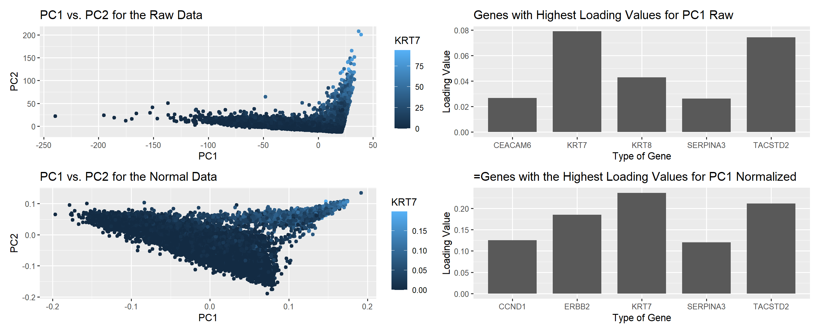
What happens if I do or not not normalize and/or transform the gene expression data (e.g. log and/or scale) prior to dimensionality reduction?
What data types are you visualizing?
I wanted to visualize quantitative data in regards to the gene expression for KRT7, and the loading values in regards to the genes with the highest loading values before and after PCA. In addition, I wanted to see the categorical data in terms of what specific genes were being regarded highly in PC1.
What data encodings (geometric primitives and visual channels) are you using to visualize these data types?
For this plot, I utilized the geometric primitive of points and area to represent each individual cell and the loading values. To encode the projection of the cells, along PC1 I utilized the x spatial position, similarily PC2 was encode in the y spatial position. In addition, the level of KRT7 expression was encoded through color saturation to indicate high vs. low levels of expression. For the loading values, I used area to encode the quantitative data as bars on a bar chart.
What about the data are you trying to make salient through this data visualization?
My data visualization seeks to make more salient the differences between non-normalized and normalized gene expression before linear dimensional reduction and the effects on the PCs and loading values specifically.
install.packages('patchwork')
install.packages('Rtsne')

data <- read.csv('pikachu.csv.gz', row.names = 1)
dim(data)
data[1:5, 1:5]

# matrix for position and gene expression
pos <- data[,4:5]
head(pos)
gexp <- data[, 6:ncol(data)]
head(gexp)

## recommend limiting the number of genes (not all genes are expressed)
# get the top 150 genes with a variance of more than 0 (is being expressed)
topgene = names(sort(apply(gexp, 2, var), decreasing = TRUE)[1:150])

# now we get all the expressions of the top genes
gexpfilter <- gexp[, topgene]

# let's try calculating the pcs with pca
pcs <- prcomp(gexpfilter)
dim(pcs$x)
plot(pcs$sdev)

# let's explore the loading values for PC1
top_loading_pc1 <- names(sort(pcs$rotation[,1], decreasing = TRUE)[1:5])
pc1_load <- data.frame(top_loading_pc1, pcs$rotation[top_loading_pc1,1])
pc1_load
dim(pc1_load)
#KRT7 > TACSTD2 > KRT8 > CEACADM6 > SERPINA3 > EPCAM

# let's plot the results for the raw data
library(ggplot2)
df_rawpcs <- data.frame(pcs$x[,1:2], KRT7 = gexpfilter[, 'KRT7'])
p1 <- ggplot(df_rawpcs) + geom_point(aes(x = PC1, y=PC2, col = KRT7)) +
  labs(title = "PC1 vs. PC2 for the Raw Data",
       x = "PC1",
       y = "PC2")

df_rawloadings <- data.frame(genes = pc1_load[,1], loadings = pc1_load[,2])
p2 <- ggplot(df_rawloadings) +
  geom_bar(aes(x = genes, y = loadings), stat = "identity", width = 0.75)+
  labs(title = "Genes with Highest Loading Values for PC1 Raw",
       x = "Type of Gene",
       y = "Loading Value")

# now let's explore the question of normalization
gexpfilter_norm <- gexpfilter/rowSums(gexpfilter)
gexpfilter_log <- log(gexpfilter_norm+1)

pcs_log <- prcomp(gexpfilter_log)

dim(pcs_log)
plot(pcs_log$sdev)

# let's explore the loading values for the normalized data
log_loading_pc1 <- names(sort(pcs_log$rotation[,1], decreasing = TRUE)[1:5])
logpc1_load <- data.frame(log_loading_pc1, pcs_log$rotation[log_loading_pc1,1])
logpc1_load
dim(logpc1_load)

# let's plot the results based on the PCA analysis
df_log <- data.frame(pcs_log$x[,1:2], KRT7 = gexpfilter_log[, 'KRT7'])
p3 <- ggplot(df_log) + geom_point(aes(x = PC1, y=PC2, col = KRT7)) +
  labs(title = "PC1 vs. PC2 for the Normal Data",
       x = "PC1",
       y = "PC2")

df_logloadings <- data.frame(genes = logpc1_load[,1], loadings = logpc1_load[,2])
p4 <- ggplot(df_logloadings) +
  geom_bar(aes(x = genes, y = loadings), stat = "identity", width = 0.75)+
  labs(title = "=Genes with the Highest Loading Values for PC1 Normalized",
       x = "Type of Gene",
       y = "Loading Value")

p1+p2+p3+p4