Performance of Nonlinear Dimensionality Reduction on Genes and PCA

Write a description of your data visualization

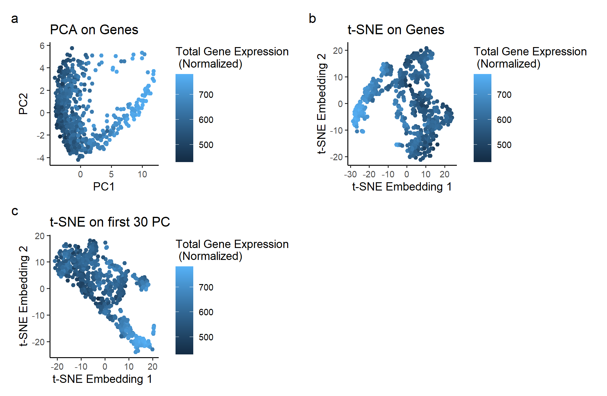
The plots use the geometric primitive of points placed according to its principal components, t-SNE Embeddings based on Gene Expression, or t-SNE Embeddings based on the principal components of the dataset. It utilizes the visual channels of color to express total gene expression at each point. Position, determined by PCA and t-SNE embeddings, is also used to organize each point based on its gene expression.

What happens if I perform non-linear dimensionality reduction on genes or PCs?

Plot a, the dataset plotted based on its first two principal components, shows a non-linear 2D plot. The PC1 seems to correspond to the total gene expression of each spot. However, PC2 is unable to encode any information on the total gene expression. If we want to find a pair of basis that allows us to see information about gene expression on both the horizontal and vertical axis, we would need to apply a non-linear dimensionality reduction techniques like t-SNE to the PCA plot.

Plot b shows what happens if t-SNE is performed on just the gene expression dataset. It is in a surprisingly similar situation as plot a, with a similar “V” shape and the same issue of only one axis corresponding to the total gene expression.

Plot c shows the results of performing t-SNE on the non-linear PCA data used for plot a. In this plot, the color changes in a diagonal direction, showing that the information on gene expression is encoded in both the vertical and horizontal axis. With non-linear dimensionality reduction, we can get two basis that both correspond to the information we want to highlight.

Please share the code you used to reproduce this data visualization.

data <- read.csv('C:\\Users\\emw\\OneDrive - Johns Hopkins\\spring 2024\\genomic-data-visualization-2024\\data\\eevee.csv.gz', row.names=1)
dim(data)
data[1:5,1:5]
pos <- data[,2:3]
gexp <- data[, 4:ncol(data)]

## recommend limiting the number of genes
?apply
topgene <- names(sort(apply(gexp, 2, var), decreasing=TRUE)[1:1000]) 
gexpfilter <- gexp[,topgene]
dim(gexpfilter)

#normalization
gexpnorm <- log10(gexpfilter/rowSums(gexpfilter) * mean(rowSums(gexpfilter))+1)

## let's try PCA
?prcomp
pcs <- prcomp(gexpnorm)
plot(pcs$sdev[1:30])

library(Rtsne)
?Rtsne
emb1 <- Rtsne(pcs$x[,1:30], dims = 2) ## what happens if we run tSNE on PCs?
emb2 <- Rtsne(gexpnorm, dims = 2)
## plot
df <- data.frame(pcs$x[,1:2], emb1=emb1$Y, emb2=emb2$Y,gene = rowSums(gexpnorm))
p1 <- ggplot(df) + geom_point(aes(x = PC1, y = PC2, col=gene)) +
  theme_classic()+ ggtitle("PCA on Genes")+
  labs(color="Total Gene Expression \n (Normalized)")

p2 <- ggplot(df) + geom_point(aes(x = emb1.1, y = emb1.2, col=gene)) +
  theme_classic()+ ggtitle("t-SNE on Genes") + 
  labs(x="t-SNE Embedding 1", y="t-SNE Embedding 2", color="Total Gene Expression \n (Normalized)")

p3 <- ggplot(df) + geom_point(aes(x = emb2.1, y = emb2.2, col=gene)) +
  theme_classic()+ ggtitle("t-SNE on first 30 PC")+ 
  labs(x="t-SNE Embedding 1 ", y="t-SNE Embedding 2", color="Total Gene Expression \n (Normalized)")

library(patchwork)
p1 + p2+p3 +plot_annotation(tag_levels = 'a')+ plot_layout(ncol = 2) + plot_layout(widths = 1)