Varying the number of principal components used to perform non-linear dimensionality reduction on barcode-based sequencing data

Description of Data Visualization
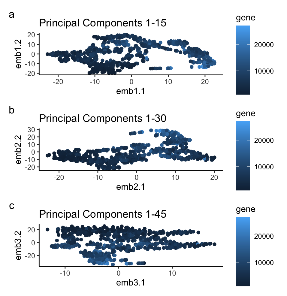
Three graphs are used to illustrate the impact of increasing the number of principal components used for non-linear dimensionality reduction. Points are used as a geometric primitive to represent each spatial barcode in the sequencing data, now visualized as a function of their highly impacting genes in two dimensions. Blue color saturatation is used to represent the gene expression at each bead. Relative position along the x and y axis represents groupings of data based on the dimensional reduction. The Gestalt principle of similarity is invoked to show similar groupings of gene expression, and proximity is used to represent the similarity in terms of the reduced variables as a function of genes.
# code taken from Dr. Fan's code-lesson-5.R
data <- read.csv('eevee.csv.gz', row.names=1)
data[1:5,1:5]
pos <- data[,2:3]
gexp <- data[, 4:ncol(data)]

# code taken from Dr. Fan's code-lesson-5.R
topgene <- names(sort(apply(gexp, 2, var), decreasing=TRUE)[1:1000])
gexpfilter <- gexp[,topgene]

# code taken from Dr. Fan's code-lesson-5.R
gexpnorm <- log10(gexpfilter/rowSums(gexpfilter) * mean(rowSums(gexpfilter))+1)

pcsnorm <- prcomp(gexpnorm)

library(Rtsne)

# code taken from Dr. Fan's code-lesson-5.R
emb1 <- Rtsne(pcsnorm$x[,1:15], dims = 2)
emb2 <- Rtsne(pcsnorm$x[,1:30], dims = 2)
emb3 <- Rtsne(pcsnorm$x[,1:45], dims = 2)

df <- data.frame(pcsnorm$x[,1:2], emb1=emb1$Y, emb2=emb2$Y, emb3=emb3$Y, gene = rowSums(gexpfilter))

# titles taken from https://ggplot2.tidyverse.org/reference/ggtheme.html
p1 <- ggplot(df) + geom_point(aes(x = emb1.1, y = emb1.2, col=gene)) + labs(title="Principal Components 1-15") + theme_classic()
p2 <- ggplot(df) + geom_point(aes(x = emb2.1, y = emb2.2, col=gene)) + labs(title="Principal Components 1-30") + theme_classic()
p3 <- ggplot(df) + geom_point(aes(x = emb3.1, y = emb3.2, col=gene)) + labs(title="Principal Components 1-45") + theme_classic()

# code taken from Dr. Fan's code-lesson-5.R
library(patchwork)
p1 + p2 + p3 + plot_annotation(tag_levels = 'a') + plot_layout(ncol = 1)