HW1 Submission: Visualizing Locations of Different Gene Expressions

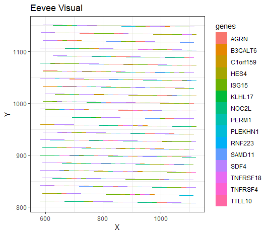
[description] For my data visualization, I analyzed 15 different genes and displayed the proportion of genes expressed in a certain spot, also showing their location. I have spatial data that I’m visualizing (x,y), as well as categorical data for each gene, and numerical data for the count of each gene in a spot. For geometric primitives, I am using points (but looks like a line) to represent each spatial data point, and area to show the genes expressed at that point and how many are expressed. For visual channels, I am using hue to show the different types of genes expressed at each point, and size to show the quantitative proportion of genes expressed at that point, and the shape of a rectangle (but looks like a line) to represent a spot. I am trying to make salient the different types of genes expressed at each spatial location and see where certain genes are more expressed than others. I used my scatterbar package (which I developed in an internship, however, I see with the vast amount of spots present, it is tough to get a clear picture, suggesting that further improvements could be made). Gestalt principles I used were similarity, with each gene associated with a hue in the scatterbar, and also continuity (at least I tried), with each spot being represented by a stacked bar chart of different colors to show the proportions adding up to 1 and what is expressed at that spot.
# Dee Velazquez
# HW 1

# Get eevee dataset
data <- read.csv('eevee.csv.gz', row.names = 1)
dim(data)
ncol(data)
data[1:10, 1:10]
colnames(data)

library(ggplot2)
library(dplyr)

#x <- data$aligned_x
#y <- data$aligned_y

# Create a pos df with x and y
pos <- data[2:3]
pos <-as.data.frame(pos)
# Rename columns to x and y
names(pos) <- c("x", "y", "spot")
# Make data a df
data <- as.data.frame(data)
# Create a column for spots
data$spot <- rownames(data)
# Create df for genes
genes<- data[, 4:ncol(data)]
# Create a df to easily view gene counts in a spot
data_long <-tidyr::pivot_longer(genes, cols = -spot, names_to = "genes", values_to = "count")
# Focus on 15 genes and repeat process
new_genes<-genes[1:15]
new_genes$spot<-rownames(new_genes)
data_long2 <-tidyr::pivot_longer(new_genes, cols = -spot, names_to = "genes", values_to = "count")
# Turn gene counts into proportions, so we can see the proportion of genes
# expressed in each spot
data_long3 <-
  data_long2 %>%
  group_by(spot) %>%
  mutate(proportion = count / sum(count)) %>%
  select(-count) %>%
  distinct()

# Combine pos and gene proportion data
# We can then use this to create a scatterbar (stacked
# bar graph at each (x,y))
combined_data <- merge(data_long3, pos, by = "spot")
combined_data <- combined_data %>%
  group_by(x, y) %>%
  # Ensures that the heights of the bars within a spot add up to 1
  mutate(cumulative_proportion = cumsum(proportion) - proportion)

# Correct positioning of bars within each (x, y) spot
p <- ggplot(combined_data, aes(x = x, y = y + cumulative_proportion + proportion/2)) +
  geom_tile(aes(fill = genes, height = proportion), width = 50, lwd = 0) +
  theme_bw() +
  labs(title = "Eevee Visual", x = "X", y = "Y")
p