Breast Glandular Cells in EEVEE Data Set
Write a description of what you changed and why you think you had to change it.
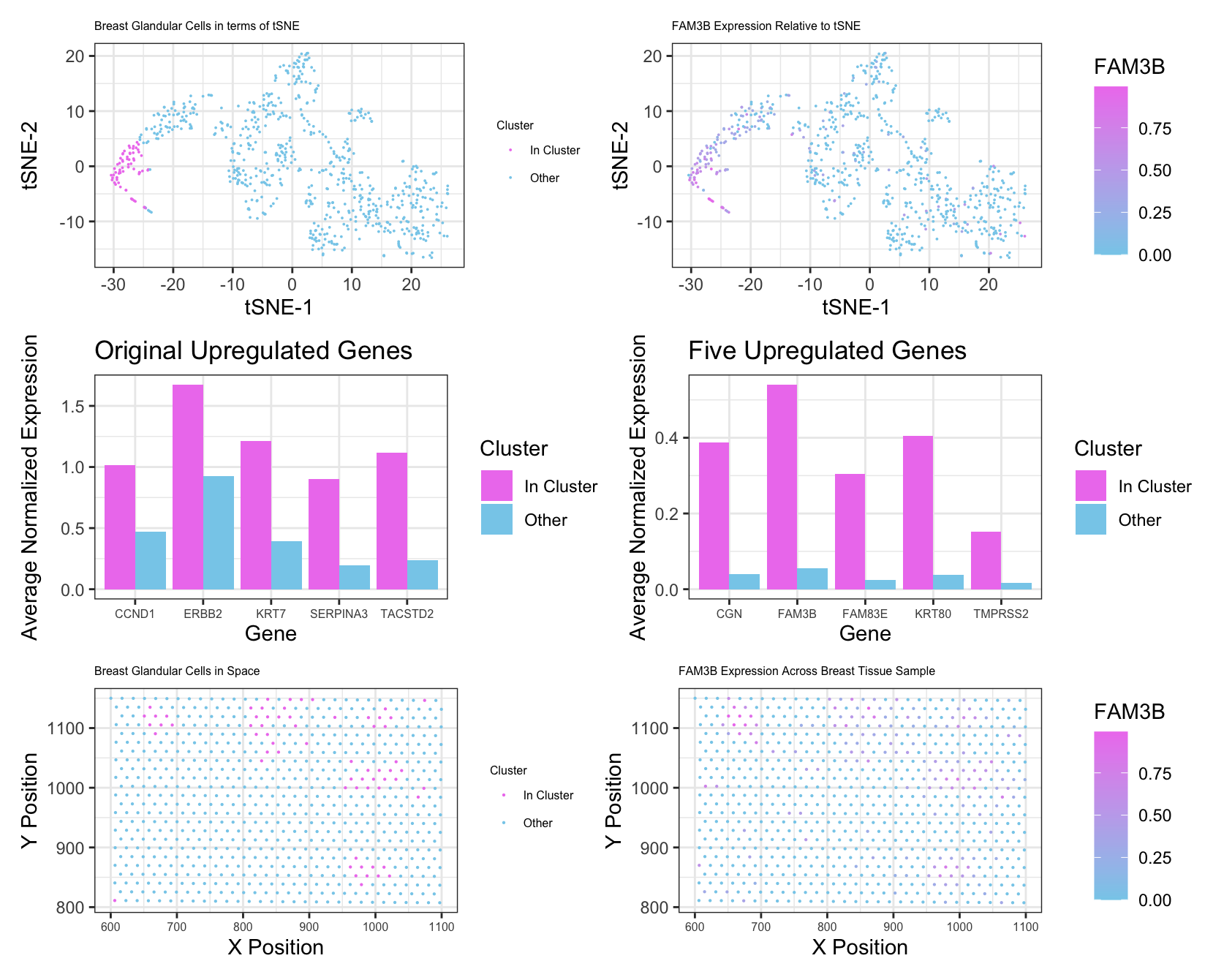
I changed my number of clusters from 7 to 8. After assessing total withiness for different k values using a loop, 8 seemed to be the best number based on the “elbow” of the graph. From this, I was able to identify a cluster that spatially aligned with the cluster I studied in the Pikachu data set. I think I had to make this change due to the number of genes contained in the EEVEE data set. With more genes being included in processes like principal component analysis and tSNE, there was more possibility for variation in gene expression from cell to cell, necessitating more groups of cells. I also did filter out some of the very minimally expressed genes prior to PCA. This was to streamline computational efficiency, as these genes wouldn’t have had a significant effect on the PCs anyways. Most of my other changes were minimal. I identified the first cluster as being my cluster of interest based on similar spatial positioning to my cluster in the Pikachu data set. After looking at the genes with the 5 smallest p values from my Wilcoxon test, I determined that these genes were all markers of breast glandular cells, which made me confident that this was a similar cluster to in the Pikachu data set. To further confirm this, I made an additional plot looking at the average expression levels of the 5 upregulated genes from my Pikachu cluster in my new cluster, and also so signficant upregulation. The last change that I made was to plot FAM3B as my gene of interest, simply because it was one fo the strongest markers for this new cluster. These changes were mostly in the interest of clarity and for confirmation of my analyis rather than out of necessity for the difference in data.
Sources: https://www.proteinatlas.org/ENSG00000143375-CGN/single+cell+type/breast https://www.proteinatlas.org/ENSG00000167767-KRT80/single+cell+type/breast https://www.proteinatlas.org/ENSG00000184012-TMPRSS2/single+cell+type/breast https://www.proteinatlas.org/ENSG00000105523-FAM83E/single+cell+type/breast https://www.proteinatlas.org/ENSG00000183844-FAM3B/single+cell+type/breast
library(ggplot2)
library(patchwork)
library(Rtsne)
library(dplyr)
library(reshape2)


data <- read.csv('eevee.csv.gz', row.names = 1)
pos <- data[,2:3]
gexp <- data[, 4:ncol(data)]
gexp <- gexp[, colSums(gexp) > 1000] ## highly expressed genes
rownames(pos) <- rownames(data) <- data$barcode
dim(gexp)

## normalizing by total gene expression
gexpnorm <- log10(gexp/rowSums(gexp) * mean(rowSums(gexp))+1)

## pca
pcs <- prcomp(gexpnorm)

## tSNE
emb <- Rtsne(pcs$x[,1:20])$Y

## determining optimal cluster number
results <- sapply(seq(2, 20, by=1), function(i) {
  print(i)
  com1 <- kmeans(pcs$x[,1:20], centers=i)
  return(com1$tot.withinss)
})
plot(results, type="l")

## final k means clustering with 7 clusters
com1 <- as.factor(kmeans(pcs$x[,1:20], centers=8)$cluster)
clusters <- data.frame(gexpnorm, pos, emb, com1)
cluster1 <- filter(clusters, com1 == 1)
other <- filter(clusters, com1 != 1)

## categorizing genes as in or out of cluster
inone <- vector('integer', 709)
for(i in 1:nrow(clusters)) {
  if(clusters$com1[i] == 1) {
    inone[i] <- 1
  }
  else {
    inone[i] <- 0
  }
}
clusters <- data.frame(clusters, inone)

## panel visualizing cluster of interest in reduced dimensional space (PCA, tSNE, etc)
p1 <- ggplot(clusters) +
  geom_point(aes(x = X1, y = X2, col = as.factor(inone)), size=0.01) +
  theme_bw() +
  scale_colour_manual(name = "Cluster", labels = c("Other", "In Cluster"), values = c("skyblue", "violet")) + xlab('tSNE-1') +
  ylab('tSNE-2') + labs(title = 'Breast Glandular Cells in terms of tSNE') +
  theme(plot.title = element_text(size = 6)) +
  guides(colour = guide_legend(reverse=TRUE)) +
  theme(legend.key.size = unit(0.5, 'cm')) +
  theme(legend.title = element_text(size=6)) +
  theme(legend.text = element_text(size=6))

## A panel visualizing your one cluster of interest in physical space
p2 <- ggplot(data.frame(pos, com1)) +
  geom_point(aes(x = aligned_x, y = aligned_y, col = as.factor(inone)), size = 0.1) +
  theme_bw() +
  scale_colour_manual(name = "Cluster", labels = c("Other", "In Cluster"), values = c("skyblue", "violet")) +
  xlab('X Position') +
  ylab('Y Position') + labs(title = 'Breast Glandular Cells in Space') +
  theme(plot.title = element_text(size = 6)) +
  guides(colour = guide_legend(reverse=TRUE)) +
  theme(legend.key.size = unit(0.5, 'cm')) +
  theme(legend.title = element_text(size=6)) +
  theme(legend.text = element_text(size=6)) +
  theme(axis.text.x=element_text(size=6))

## Wilcox test to determine most up-regulated genes
g = 'CD79A'
gexpnorm[com1 == 1, g]
results <- sapply(colnames(gexpnorm), function(g) {
  wilcox.test(gexpnorm[com1 == 1, g],
              gexpnorm[com1 != 1, g],
              alternative = "greater")$p.val
})
results
sort(results, decreasing=FALSE)


## identifying genes w/ smallest p-vals
topgenes <- as.data.frame(sort(results, decreasing=FALSE)[1:5])
topgeneexp <- data.frame(matrix(ncol = 3, nrow = 5))
colnames(topgeneexp) <- c('gene','clusterexp','otherexp')

## genes from pikachu
firstfive <- data.frame('KRT7','TACSTD2','ERBB2','SERPINA3','CCND1')
colnames(firstfive) <- c('KRT7','TACSTD2','ERBB2','SERPINA3','CCND1')
fivegeneexp <- data.frame(matrix(ncol = 3, nrow = 5))
colnames(fivegeneexp) <- c('gene','clusterexp','otherexp')

for(i in 1:5) {
  fivegeneexp$gene[i] <- colnames(firstfive)[i]
  fivegeneexp$clusterexp[i] <- mean(gexpnorm[com1 == 1, colnames(firstfive[i])])
  fivegeneexp$otherexp[i] <- mean(gexpnorm[com1 != 1, colnames(firstfive[i])])
}
mean(gexpnorm[com1 == 1, colnames(firstfive[i])])

## finding average normalized expression of top genes in vs out of cluster
for(i in 1:nrow(topgenes)) {
  topgeneexp$gene[i] <- rownames(topgenes)[i]
  topgeneexp$clusterexp[i] <- mean(gexpnorm[com1 == 1, rownames(topgenes)[i]])
  topgeneexp$otherexp[i] <- mean(gexpnorm[com1 != 1, rownames(topgenes)[i]])
}


## A panel visualizing differentially expressed genes for your cluster
topgenesorted <- topgeneexp[order(topgeneexp$clusterexp, decreasing = TRUE),]
topfive <- topgenesorted[1:5,]
df2 <- melt(topfive, id.vars='gene')
p3 <- ggplot(df2, aes(x=gene, y=value, fill=variable)) +
  geom_bar(stat='identity', position='dodge') +
  scale_fill_manual(name = 'Cluster', labels = c("In Cluster", "Other"), values = c("violet", "skyblue")) +
  labs(title = "Five Upregulated Genes") + xlab('Gene') +
  ylab('Average Normalized Expression') +
  theme(plot.title = element_text(size = 6)) +
  theme_bw() +
  theme(axis.text.x=element_text(size=6))

## Original 5
df3 <- melt(fivegeneexp, id.vars='gene')
p6 <- ggplot(df3, aes(x=gene, y=value, fill=variable)) +
  geom_bar(stat='identity', position='dodge') +
  scale_fill_manual(name = 'Cluster', labels = c("In Cluster", "Other"), values = c("violet", "skyblue")) +
  labs(title = "Original Upregulated Genes") + xlab('Gene') +
  ylab('Average Normalized Expression') +
  theme(plot.title = element_text(size = 6)) +
  theme_bw() +
  theme(axis.text.x=element_text(size=6))


## A panel visualizing one of these genes in reduced dimensional space
p4 <- ggplot(data.frame(emb, gexpnorm)) +
  geom_point(aes(x= X1, y = X2, col = FAM3B), size = 0.01 ) +
  scale_colour_gradientn(colours = c("skyblue", "violet"))+
  labs(title = "FAM3B Expression Relative to tSNE") + xlab('tSNE-1') +
  ylab('tSNE-2') +
  theme_bw() +
  theme(plot.title = element_text(size = 6))

## A panel visualizing one of these genes in space
p5 <- ggplot(data.frame(pos, gexpnorm)) +
  geom_point(aes(x = aligned_x, y = aligned_y, col = FAM3B), size = 0.1) +
  scale_colour_gradientn(colours = c("skyblue", "violet"))+
  labs(title = "FAM3B Expression Across Breast Tissue Sample") + xlab('X Position') +
  ylab('Y Position') +
  theme_bw() +
  theme(plot.title = element_text(size = 6)) +
  theme(axis.text.x=element_text(size=6))


p5
top <- p1 + p4
mid <- p6 + p3
bottom <- p2 + p5
full <- top/mid/bottom
full