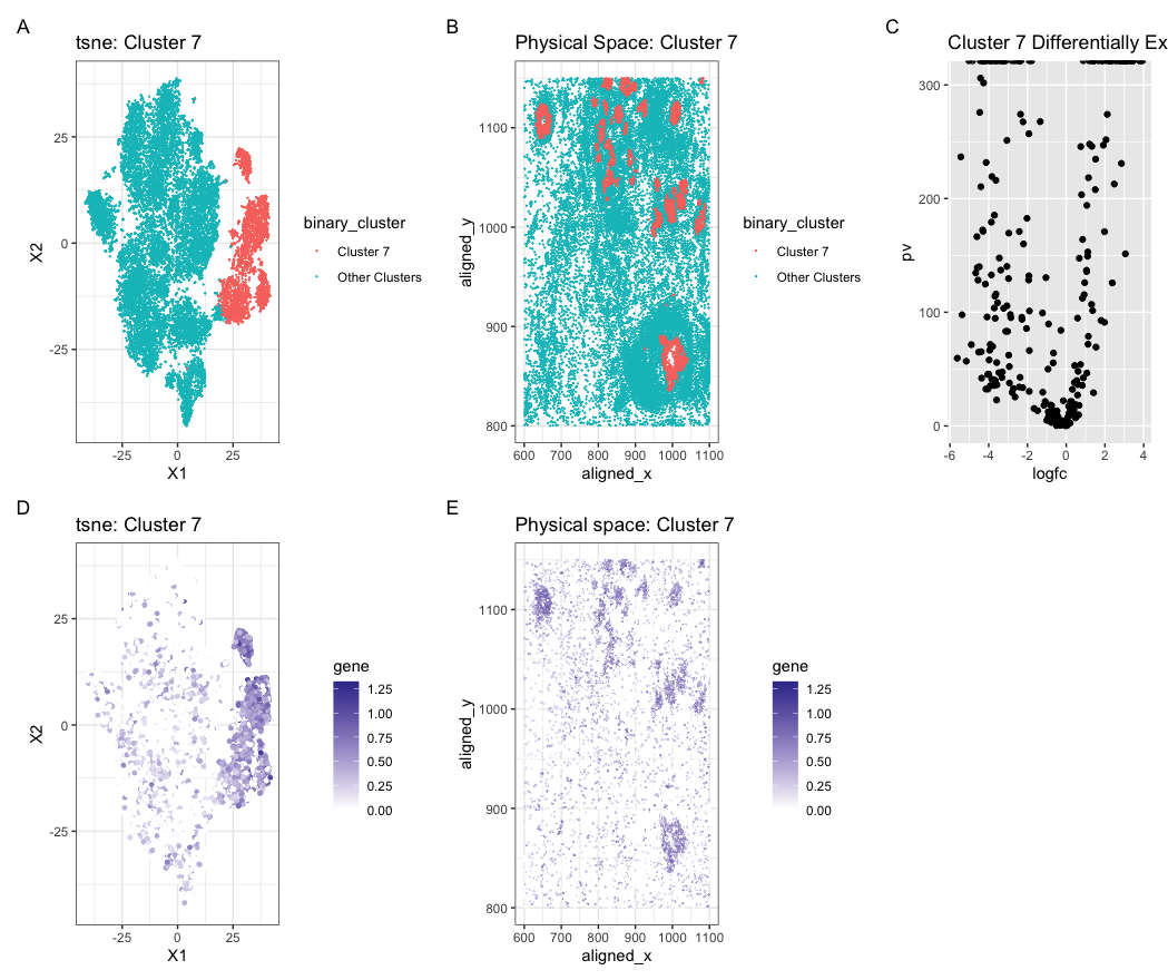
Expression of CD9 in reduced dimensional and physical space

Create a multi-panel data visualization and write a description to convince me you found the same cell-type.
In my original Eevee dataset, I identified a cell cluster that differentially expressed the gene MMP7 which is a gene that is normally upregulated in epithelial and cancer cells. When running the code, finding the expression fro MMP7 resulted in an error. I then did a little outside research to find other marker genes for breast cancer and epethelial cells and found that CD9 is a marker gene. This provides me with strong evidence that the cluster I have identified in the Pikachu dataset is the same cell type I identified in the Eevee dataset.
Write a description of what you changed and why you think you had to change it
I adjusted the pos and gexp variables to correspond with the columns in the pikachu dataset as opposed to the eevee dataset. Additionally, I also changed the gene of interest because my initial gene of interest yielded errors in the code. I also adjusted which cluster I was interested in that matched my gene of interest to ensure I had the correct cell type.
#install.packages('Rtsne')
#install.packages('ggplot2')

library(Rtsne)
library(ggplot2)
library(patchwork)

data <- read.csv('/Users/conniechen/Documents/Genomic Data Visualization 2024/GDV HW/pikachu.csv.gz', row.names = 1)
dim(data)

pos <- data[, 4:5]
gexp <- data[6:ncol(data)] ### Adjusted pos and gexp to apply for pikachu dataset
### Defining additional variables
rownames(pos) <- rownames(gexp) <- data$cell_id
cell_area <- data$cell_area
names(cell_area) <- data$cell_id
head(cell_area)

### Limit the number of genes
# subset for faster processing
gexp <- gexp[, colSums(gexp) > 1000] ## highly expressed genes
# probably also normalize...
gexpnorm <- log10(gexp/rowSums(gexp) * mean(rowSums(gexp))+1)
#com <- as.factor(kmeans(gexpnorm, centers=10)$cluster)


### PCA
pcs <- prcomp(gexpnorm)
dim(pcs$x)
plot(pcs$sdev[1:100])

### tsne
emb <- Rtsne(pcs$x[,1:20])$Y


### Kmeans clustering and tsne plotting
com <- as.factor(kmeans(gexpnorm, centers=10)$cluster)

### Changing cluster colors

## help from chatgpt
binary_cluster <- ifelse(com == 7, "Cluster 7", "Other Clusters")
binary_cluster <- as.factor(binary_cluster)

### plotting tsne cluster 7
p1 <- ggplot(data.frame(emb, binary_cluster), aes(x = X1, y = X2, col=binary_cluster)) +
  geom_point(size=0.05) +
  theme_bw() +
  ggtitle('tsne: Cluster 7')
  scale_color_manual(values = c("Cluster 7" = "light green", "Other Clusters" = "dark blue"))

### plotting physical space cluster 7
p2 <- ggplot(data) + geom_point(aes(x = aligned_x, y = aligned_y, col = binary_cluster), size = 0.05) +
  theme_bw() +
  ggtitle('Physical Space: Cluster 7')
  scale_color_manual(values = c("Cluster 7" = "light blue", "Other Clusters" = "light blue"))

p1 + p2
### pv versus log fc

pv <- sapply(colnames(gexpnorm), function(i) {
  #print(i) ## print out gene name
  wilcox.test(gexpnorm[com == 7, i], gexpnorm[com != 7, i])$p.val
})
logfc <- sapply(colnames(gexpnorm), function(i) {
  #print(i) ## print out gene name
  log2(mean(gexpnorm[com == 7, i])/mean(gexpnorm[com != 7, i]))
})

df <- data.frame(pv=-log10(pv), logfc)
p3 <- ggplot(df) + geom_point(aes(x = logfc, y = pv)) + ggtitle('Cluster 7 Differentially Expressed Genes')

p1 + p2 + p3

### tsne for gene CD9

geneclusters <- as.factor(kmeans(t(gexpnorm), centers=10)$cluster)
head(geneclusters[geneclusters == 7])

df2 <- data.frame(emb, gene=gexpnorm[, 'CD9'])
df3 <- data.frame(pos, gene = gexpnorm[, 'CD9'])
p4 <- ggplot(df2) + geom_point(aes(x = X1, y = X2, col=gene), size=1) +
  theme_bw() +
  ggtitle('tsne: Cluster 7') +
  scale_color_gradient2(high = scales::muted("blue"), mid = 'white', low = scales::muted("red"))

### Cluster 7 in physical space

p5 <- ggplot(df3) + geom_point(aes(x = aligned_x, y = aligned_y, col=gene), size=0.05) +
  theme_bw() +
  ggtitle('Physical space: Cluster 7') +
  scale_color_gradient2(high = scales::muted("blue"), mid = 'white', low = scales::muted("red"))

p1 + p2 + p3 + p4 + p5 + plot_annotation(tag_levels = 'A')