Locating a cell type in breast tissue using spatial transcriptomics data

Describe your figure briefly so we know what you are depicting (you no longer need to use precise data visualization terms as you have been doing).
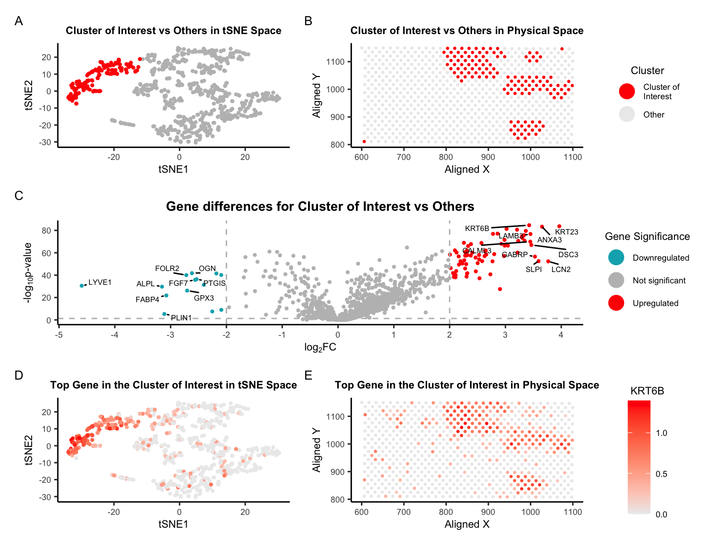
There are five plots in this figure. Plot A shows the tSNE space with the cluster of interest in red and all other clusters in gray. Clusters were determined using the kmeans algorithm with k=5 clusters. Plot B shows the physical space (i.e. the 10x Visium spots located on the tissue) with the cluster of interest in red and all other clusters in gray. Plot C shows a volcano plot of the gene differences for the cluster of interest vs all other clusters. Here, genes in red are upregulated, genes in blue are downregulated, and genes in gray are not significant when taking into account p-values and a fold change greater than 2 or less than -2. The names of the top 20 genes based on the thresholds mentioned are printed within the plot. Genes were determined to be significant based on their pvalue from the two-sided Wilcoxon Rank Sum test. Plot D shows the tSNE space with the top gene found from DE analysis, KRT6B, in the cluster of interest as a gradient from gray to red. Plot E shows the physical space with KRT6B expression in the cluster of interest also as a gradient from gray to red.
Write a description to convince me that your cluster interpretation is correct. Your description may reference papers and content that allowed you to interpret your cell cluster as a particular cell-type. You must provide attribution to external resources referenced. Links are fine; formatted references are not required.
After some research, I’ve decided that my cluster of interest best corresponds to glandular epithelial cells within the breast tissue sample. This is based on the expression of the genes KRT6B, KRT17, and KRT23 which are known to be highly expressed in this cell type and are three out of the top five DE genes based on the Wilcoxon Rank Sum test. KRT6B is a member of the keratin gene family, which are intermediate filament proteins that are expressed in glandular epithelial cells [1] along with KRT17 [2]. KRT23 is another member of the keratin gene family and responsible for the structural integrity of epithelial cells [3]. Further, there are countless studies that have shown that these genes are not only expressed on breast tissue but are related to the diagnosis and prognosis of breast cancer. Reduced expression of KRT17 was shown to predict a poor prognosis in HER2-high breast cancer [4]. One preprint in 2022 declared that KRT6B expression is significantly higher in basal-like breast cancers [5]. Hence, I’d be curious to know what type of breast cancer this is… Finally, there are a handful of papers relating KRT23 to breast cancer but one in particular notes that high expression levels of KRT23 (along with NCCRP1) indicated high proliferation and poor prognosis. The title of this paper states the authors believe that the combined targeting of KRT23 and NCCRP1 could be a potential novel therapeutic approach for the treatment of triple-negative breast cancer [6]. Overall, these three genes are known the be highly expressed in glandular epithelial cells and are related to breast cancer, which is why I believe my cluster of interest is glandular epithelial cells within the breast tissue sample.
References
[1] https://www.ncbi.nlm.nih.gov/gene/3854
[2] https://www.ncbi.nlm.nih.gov/gene/3872
[3] https://www.genecards.org/cgi-bin/carddisp.pl?gene=KRT23
[4] https://www.ncbi.nlm.nih.gov/pmc/articles/PMC9496156/
[5] https://osf.io/preprints/osf/nsker
[6] https://pubmed.ncbi.nlm.nih.gov/36353580/
Code
### HW4 ###
## Caleb Hallinan ##
## Eevee sequencing data ##

# import libraries
library(here)
library(ggplot2)
library(Rtsne)
library(patchwork)
library(factoextra)
library(ggrepel)

# set seed
set.seed(02052024)


#### Data Preprocessing ####

# read in data
data = read.csv(here("data/eevee.csv.gz"), row.names = 1)
# dim(data)
# get info from data
pos <- data[,2:3]
gexp <- data[,4:ncol(data)]
# colnames(gexp)
# check variance
topgenes <- names(sort(apply(gexp, 2, var), decreasing=TRUE)[1:2000])
topgenes
# filter
gexpfilter <- gexp[,topgenes]
# normalize log2
gexpnorm <- log10(gexpfilter/rowSums(gexpfilter) * mean(rowSums(gexpfilter))+1)


#### Dimensionality Reduction ####

# perform pca
pcs <- prcomp(gexpnorm)

# run tsne on top PCs
set.seed(02052024)
emb <- Rtsne(pcs$x[,1:20], perplexity = 15) # can change dims from
# names(emb)

# gene to plot
gene <- topgenes[3]

# plot tsne to see
# ggplot(data.frame(emb$Y)) +
#     geom_point(aes(x = emb$Y[,1], y = emb$Y[,2], color =clusters)) +
#     theme_classic() +
#     labs(
#         title = "tSNE on Top 1000 Genes with High Variance",
#         color = gene,
#         x = "tSNE1",
#         y = "tSNE2"
#     ) +
#     # scale_color_gradient2(midpoint = median(gexpnorm[[gene]]), low = "blue", mid = "#ECECEC", high = "red", space = "Lab" ) +
#     theme(legend.title.align=0.5,plot.title = element_text(hjust = 0.5, face="bold", size=14), text = element_text(size = 13))


#### Clustering ####

#create plot of number of clusters vs total within sum of squares
# fviz_nbclust(data.frame(emb$Y), kmeans, method = "wss")

# perform kemans clustering based on elbow plot
set.seed(02052024)
clusters <- as.factor(kmeans(emb$Y, 5)$cluster)

# get just cluster of interest
cluster_of_interest <- ifelse(clusters == 4, "Cluster of\nInterest", "Other")

# plot tsne to see
# ggplot(data.frame(emb$Y)) +
#     geom_point(aes(x = emb$Y[,1], y = emb$Y[,2], color = clusters), size=0.75) +
#     theme_classic() +
#     labs(
#         title = "Clusters in tSNE Space",
#         color = "Cluster",
#         x = "tSNE1",
#         y = "tSNE2"
#     ) +
#     # scale_color_gradient2(midpoint = median(gexpnorm[[gene]]), low = "blue", mid = "#ECECEC", high = "red", space = "Lab" ) +
#     theme(legend.title.align=0.5,plot.title = element_text(hjust = 0.5, face="bold", size=8), text = element_text(size = 8)) +
#     guides(color = "none")


#### DE Gene Analysis ####

# do wilcox for DE genes
pv <- sapply(colnames(gexpnorm), function(i) {
    print(i) ## print out gene name
    wilcox.test(gexpnorm[clusters == 4, i], gexpnorm[clusters != 4, i])$p.val
})

head(sort(pv))

# get log fold change
logfc <- sapply(colnames(gexpnorm), function(i) {
    print(i) ## print out gene name
    log2(mean(gexpnorm[clusters == 4, i])/mean(gexpnorm[clusters != 4, i]))
})


### Plotting ###

# gene to plot
gene <- names(sort(pv)[1])

# plot tsne to see
bottom1 <- ggplot(data.frame(emb$Y)) +
    geom_point(aes(x = emb$Y[,1], y = emb$Y[,2], color = gexpnorm[[gene]]), size=0.75) +
    theme_classic() +
    labs(
        title = "Top Gene in the Cluster of Interest in tSNE Space",
        color = gene,
        x = "tSNE1",
        y = "tSNE2"
    ) +
    scale_color_gradient2(midpoint = median(gexpnorm[[gene]]), low = "blue", mid = "#ECECEC", high = "red", space = "Lab" ) +
    theme(legend.title.align=0.5,plot.title = element_text(hjust = 0.5, face="bold", size=8), text = element_text(size = 8)) +
    guides(color = "none")


bottom2 <- ggplot(data) +
    geom_point(aes(x = aligned_x, y = aligned_y, color = gexpnorm[[gene]]), size=.5) +
    scale_color_gradient(low = "#ECECEC", high = "red", space = "Lab" ) +
    # scale_color_gradient2(midpoint = max(gexpnorm[[gene]])/2, low = "blue", mid = "#ECECEC", high = "red", space = "Lab" ) +
    theme_classic() +
    labs(
        title = "Top Gene in the Cluster of Interest in Physical Space",
        color = gene,
        x = "Aligned X",
        y = "Aligned Y"
    ) +
    guides(size = "none") +
    theme(legend.title.align=0.5,plot.title = element_text(hjust = 0.5, face="bold", size=8),
          text = element_text(size = 8))


top1 <- ggplot(data.frame(emb$Y)) +
    geom_point(aes(x = emb$Y[,1], y = emb$Y[,2], color = cluster_of_interest), size=0.75) +
    scale_color_manual(values = c("red","gray")) +
    theme_classic() +
    labs(
        title = "Cluster of Interest vs Others in tSNE Space",
        color = "Cluster",
        x = "tSNE1",
        y = "tSNE2"
    ) +
    # scale_color_gradient2(midpoint = median(gexpnorm[[gene]]), low = "blue", mid = "#ECECEC", high = "red", space = "Lab" ) +
    theme(legend.title.align=0.5,plot.title = element_text(hjust = 0.5, face="bold", size=8), text = element_text(size = 8)) +
    guides(color = "none")


top2 <- ggplot(data) +
    geom_point(aes(x = aligned_x, y = aligned_y, color = cluster_of_interest), size=0.5) +
    scale_color_manual(values = c("red","#ECECEC")) +
    # scale_color_gradient2(midpoint = max(gexpnorm[[gene]])/2, low = "blue", mid = "#ECECEC", high = "red", space = "Lab" ) +
    theme_classic() +
    labs(
        title = "Cluster of Interest vs Others in Physical Space",
        color = "Cluster",
        x = "Aligned X",
        y = "Aligned Y"
    ) +
    guides(size = "none",color = guide_legend(override.aes = list(size=5))) +
    theme(legend.title.align=0.5, plot.title = element_text(hjust = 0.5, face="bold", size=8),
          text = element_text(size = 8))


# volcano plot
df <- data.frame(pv=-log10(pv), logfc)
# add gene names
df$genes <- rownames(df)
# add labeling
df$delabel <- ifelse(df$logfc > 3.4, df$genes, NA)
df$delabel <- ifelse(df$logfc < -2.5, df$genes, df$delabel)
# add if DE
df$diffexpressed <- ifelse(df$logfc > 2, "Upregulated", "Not Significant")
df$diffexpressed <- ifelse(df$logfc < -2, "Downregulated", df$diffexpressed)

# plot
mid <- ggplot(df, aes(x = logfc, y = pv, label = delabel, color = diffexpressed)) +
    geom_point(size= 0.75) +
    geom_vline(xintercept = c(-2, 2), col = "gray", linetype = 'dashed') +
    geom_hline(yintercept = -log10(0.05), col = "gray", linetype = 'dashed') +
    scale_color_manual(values = c("#00AFBB", "grey", "red"),
                       labels = c("Downregulated", "Not significant", "Upregulated")) +
    # theme
    theme_classic() +
    # labels
    labs(color = 'Gene Significance',
         x = expression("log"[2]*"FC"),
         y = expression("-log"[10]*"p-value"),
         title = "Gene differences for Cluster of Interest vs Others") +
    theme(
        plot.title = element_text(hjust = 0.5, face="bold", size=10),
        text = element_text(size = 8)
    ) +
    geom_text_repel(max.overlaps = Inf, box.padding = 0.25, point.padding = 0.25, min.segment.length = 0, size = 2, color = "black") +
    scale_x_continuous(breaks = seq(-5, 5, 1)) +
    guides(size = "none",color = guide_legend(override.aes = list(size=5)))


# plot using patchwork
(top1 + top2) / (mid) / (bottom1 + bottom2) + plot_annotation(tag_levels = 'A')