KRT8 Expression in Breast Cancer

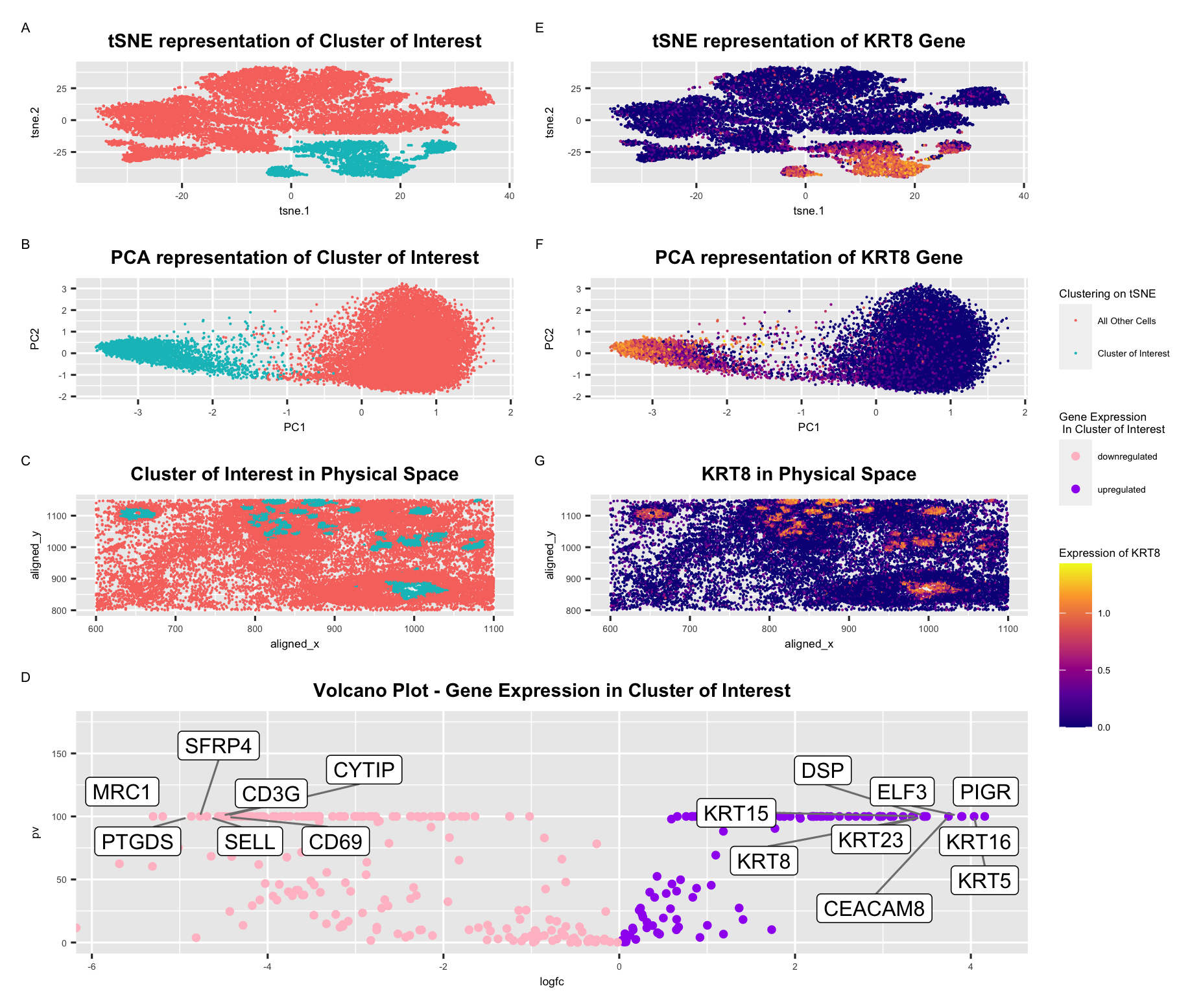
In this visualization, I explore the expression of KRT8, a cancer related gene, in breast cancer tissue. In panel A and E, I use points to represent cells in a tSNE non-linear dimensionality reduction. After running a k-means clustering analysis with 5 clusters, I used hue to separate my cluster of interest. I also showed the expression of KRT8 using a saturation gradient. In panels B and F, I show a similar dimensionality reduction using principal components analysis, representing the cells as points on a plot where the axes are the principle components. I found that there was high separation between by cluster of interest and all other cells on PC1 and explored high loading values. Similar to the tSNE plots, I used hue to separate my cluster of interest on panel B and a saturation gradient to show gene expression levels in panel F. The third row shows a reprsentation of my cells of interest in physical space, where you can see the cells of interest in teal. The expression of KRT8 is also high in similar areas as represented in panel G by the saturation gradient. The final plot, panel D, shows the differentially expressed genes in my cluster of interest. Each point reprsents a gene, and I used color to easily distinguish between downregulated and upregulated genes. This volcano plot compares the p-value resulting from a wilcoxon rank statistical test and the fold change, which is the ratio of expression levels between the two conditions. Furthermore, I labeled points with significant differential expression of genes.
Using the Human Protein Atlas, I explored the KRT8 gene, which had high negative loading on PC1 and significantly upregulated expression according to my wilcox test. I hypothesize that the cluster of interest represents cancerous breast glandular epithelial cells because this cell type in breast tissue has high expression of the KRT8 cancer gene. KRT8 is a low cancer specificity gene, so without prior knowledge of tissue sample type, I would not be able to confirm what types of cells are identified. However, when exploring the expressio in single cells and tissues, I found that KRT8 is upregulated in breast glandular cells and tissues. It is also highly expressed in breast myoepithelial cells and T-cells. I further explored breast tissue by looking at labeled tissue cross sections, and the glandular epithelial cells have a similar spatial orientation in identifiable features in my spatial plots. I would need to do more testing and potentially confirm with other genes, but my initial hypothesis is that my cluster of interest represents cancerous breast glandular epithelial cells.
Sources: https://www.proteinatlas.org/ENSG00000170421-KRT8/single+cell+type https://www.proteinatlas.org/ENSG00000170421-KRT8/tissue+cell+type
I referenced the following source when I was deciding which gene to visualize: https://www.cancergeneticsjournal.org/article/S0165-4608(07)00335-4/abstract
#HW4
#Andrea Cheng (acheng41)

#import libraries

library(ggplot2)
library(patchwork)
library(Rtsne)
library(ggrepel)
my_theme = theme(
  plot.title = element_text(hjust = 0.5, face="bold", size=10),
  text = element_text(size = 8)
)

#Load data
data = read.csv("~/Desktop/GDV class/data/pikachu.csv.gz", row.names = 1)

pos = data[,4:5]
gexp = data[,6:ncol(data)]

#normalize
gexpnorm = log10(gexp/rowSums(gexp) * mean(rowSums(gexp)) + 1)

#pca
pcs = prcomp(gexpnorm)
plot(pcs$sdev[1:40])

#tsne
emb = Rtsne(pcs$x[,1:20])$Y #faster w/ pcs which represent genes than tSNE on genes
df_tsne = data.frame(emb)

#check tsne plot
ggplot(df_tsne) + geom_point(aes(x = X1, y = X2)) + theme_classic()


#find optimal clustering coefficient k on tSNE
#look at different tot.within-ness for different k
results <- sapply(2:15, function(i){
  com <- kmeans(emb, centers = i)
  return(com$tot.withinss)
})
plot(results, type = 'l')

#kmeans with k=5
com = kmeans(emb, centers = 5)

#visualize clusters
df_clusters = data.frame(pos, tsne = emb, kmeans = as.factor(com$cluster))
df_pcs = data.frame(pcs = pcs$x, kmeans = as.factor(com$cluster))


#Main focus on Cluster #2 (consistently clustered together with various k's)
#may need to change cluster # in each run of this code

# A panel visualizing your one cluster of interest in reduced dimensional space - tSNE
fin_tsne = ggplot(df_clusters) +
  geom_point(aes(x=tsne.1, y = tsne.2,
                 col = ifelse(kmeans == 2, "Cluster of Interest", "All Other Cells")),
             size = 0.01)+
  labs(col = "Clustering on tSNE",
       title = "tSNE representation of Cluster of Interest") + my_theme

# A panel visualizing your one cluster of interest in reduced dimensional space - PCA
fin_pcs = ggplot(df_pcs) +
  geom_point(aes(x=pcs.PC1, y = pcs.PC2,
                 col = ifelse(kmeans == 2, "Cluster of Interest", "All Other Cells")),
             size = 0.01) +
  labs(col = "Clustering on tSNE",
      title = "PCA representation of Cluster of Interest")+ my_theme +
  xlab("PC1") + ylab("PC2")


# A panel visualizing your one cluster of interest in physical space
fin_tissue = ggplot(df_clusters) +
  geom_point(aes(x=aligned_x, y = aligned_y,
                 col = ifelse(kmeans == 2, "Cluster of Interest", "All Other Cells")),
             size = 0.01) +
  labs(col = "Clustering on tSNE",
      title = "Cluster of Interest in Physical Space") + my_theme


# A panel visualizing differentially expressed genes for your cluster of interest
com_categories = as.factor(com$cluster)
pv = sapply(colnames(gexpnorm), function(i){
  print(i)
  wilcox.test(gexpnorm[com_categories==2, i], gexpnorm[com_categories!=2, i])$p.val
})

logfc = sapply(colnames(gexpnorm), function(i){
  print(i)
  log2(mean(gexpnorm[com_categories==2, i])/mean(gexpnorm[com_categories!=2, i]))
})


#create a volcano plot
df_volcano = data.frame(pv=-(log10(pv+1e-100)),logfc)
#add genes as a column
df_volcano$genes <- rownames(df_volcano)
rownames(df_volcano) <- NULL
head(df_volcano)

fin_diffexp = ggplot(df_volcano) + geom_point(aes(x = logfc, y = pv, col = ifelse(logfc > 0,'upregulated', 'downregulated'))) +
  geom_label_repel(aes(x = logfc, y = pv, label=ifelse( pv == 100 & (logfc < -4.5 | logfc >3.4), as.character(genes),NA)),
                   box.padding   = 0.35, point.padding = 0.5, segment.color = 'grey50',
                   max.overlaps = getOption("ggrepel.max.overlaps", default = 60)
                   )+ ylim(-.05, 175) + labs(
                     col = "Gene Expression \n In Cluster of Interest",
                     title = "Volcano Plot - Gene Expression in Cluster of Interest"
                   ) + scale_color_manual(values = c("pink", "purple"))+ my_theme


#Show genes with high loading on PC1
pc1_high = sort(pcs$rotation[,1], decreasing = FALSE)[1:14]

#Find Genes that are high loading in PC1 and also highly differential (high pv)
top_diff_pc = Reduce(intersect,list(names(pc1_high),colnames(gene_diff)))
print(top_diff_pc)


# A panel visualizing one of these genes in reduced dimensional space- tSNE
df_KRT8 = data.frame(pos, tsne = emb, kmeans = as.factor(com$cluster), pcs = pcs$x, KRT8 = gexpnorm['KRT8'])
fin_KRT8tsne = ggplot(df_KRT8) +
  geom_point(aes(x=tsne.1, y = tsne.2,
                 col = KRT8)   ,
             size = 0.01) +
  labs(col = "Expression of KRT8",
       title = "tSNE representation of KRT8 Gene") +
  scale_color_viridis_c('Expression of KRT8', option="C") + my_theme

# A panel visualizing one of these genes in reduced dimensional space- PCA
fin_KRT8pcs = ggplot(df_KRT8) +
  geom_point(aes(x=pcs.PC1, y = pcs.PC2,
                 col = KRT8),
             size = 0.01) +
  labs(col = "Expression of KRT8",
       title = "PCA representation of KRT8 Gene") +
  scale_color_viridis_c('Expression of KRT8', option="C") + my_theme +
  xlab("PC1") + ylab("PC2")

# A panel visualizing one of these genes in space
fin_KRT8tissue = ggplot(df_KRT8) +
  geom_point(aes(x=aligned_x, y = aligned_y,
                 col = KRT8),
             size = 0.01) +
  labs(col = "Clustering on tSNE",
       title = "KRT8 in Physical Space") +
  scale_color_viridis_c('Expression of KRT8', option="C") + my_theme


#display panels
fin_tsne + fin_pcs + fin_tissue + fin_diffexp +
fin_KRT8tsne + fin_KRT8pcs + fin_KRT8tissue + plot_annotation(tag_levels = 'A')+
  plot_layout(widths = c(5, 5, 5),
                          guides = "collect",
                          design = "
              15
              26
              37
              44
              44
              ")