Cell type exploration using differential gene expression analyses

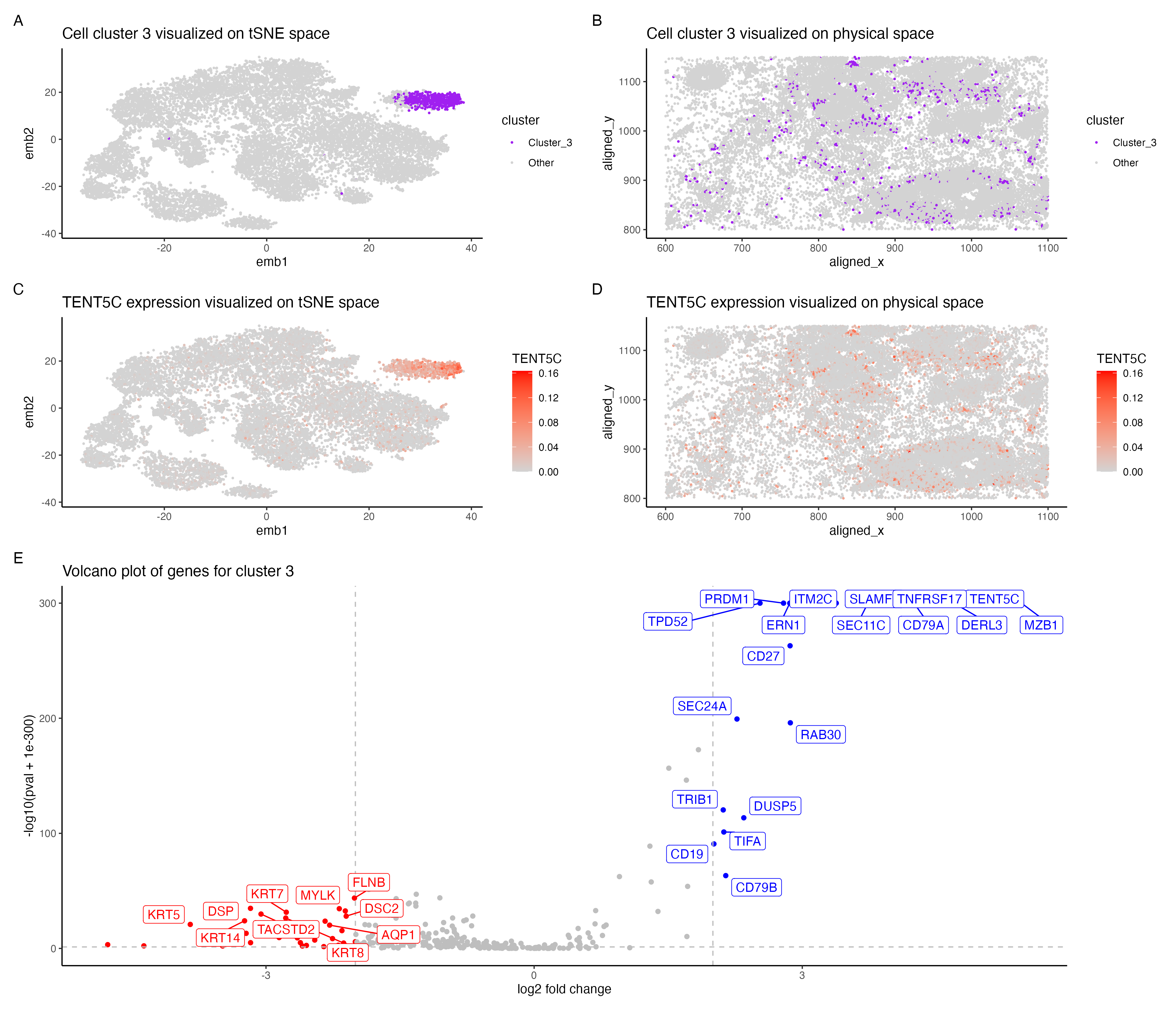
In the above visualization I have identified a cluster that belong to plasma cells or mature B cells. I started with normalizing the gene expression data by the total gene count. To perform k-means clustering I iteratively computed the total withinness score for different values of k and found 11 clusters to be an optimal number for the pikachu dataset. I then picked cluster 3 for differential gene expression analyses. Panel A shows cluster 3 in the lower dimensional space (tSNE) and panel B shows cluster 3 in the spatial dimension. Further I performed differential gene expression analyses using a Wilcoxon rank sum test, comparing cluster 3 with the rest of the cells. Panel E shows a volaco plot with log2 fold change on the x axis and -log10(pval +1e-300) on the y-axis. The points in red show significantly down regulated genes (log2fc < -2 and p < 0.05) and points in bIue show significantly upregulated genes (log2fc > 2 and p < 0.05) then visualized TENT5C gene which was significantly upregulated in cluster 3.Panel C shows expression of TENT5C in the lower dimensional space (tSNE) and panel D shows TENT5C expression in the spatial dimension.
Identifying cell type of cluster 3 The volcano plot in panel E shows that MZB1, CD79A, TENT5C, DERL3 , TNFRSF17 are significantly upregulated in cells in cluster 3. The upregulation of these genes indicates that cells potentially belong to plasma cells or mature B cells. The human protein atlas shows that these genes are most highly expressed in plasma cells followed by B cells[1]. Plasma cells are formed from activated/mature B cells and are responsible for the first line of immune response. TENT5C gene is highly expressed in plasma cells as well as activated B cells which eventually form plasma cells [2]. DERL3 and MZB1 were reported as gene markers for plasma cells from a study of whole transcriptional analysis of RNA sequencing data [3]. MZB1 is also shown to be highly expressed in marginal zone B or B1 cells[4] TNFRSF17 has also been reported as an important gene marker for plasma cells [5] and is known to be highly expressed in mature B cells [6].CD79A is shown to be expressed though all stages of B cell maturation [7]. Hence the cells in cluster 3 most likely belong to plasma cells or mature B cells.
References: [1] https://www.proteinatlas.org/humanproteome/single+cell+type [2] https://www.nature.com/articles/s41467-020-15835-3 [3] https://translational-medicine.biomedcentral.com/articles/10.1186/s12967-020-02220-3 [4] https://www.nature.com/articles/s41598-020-78293-3 [5] https://www.biocompare.com/Editorial-Articles/585833-A-Guide-to-Plasma-Cell-Markers/ [6] https://www.ncbi.nlm.nih.gov/gene/608 [7] https://pubmed.ncbi.nlm.nih.gov/7632952/
library(dplyr)
library(tidyverse)
library(ggplot2)
library(Rtsne)
library(patchwork)
library(viridis)
library(ggrepel)

set.seed(123)
## Data Description
# Each row is a cell ~17000
# Columns are mainly genes ~300

# Set working directory path and read in data
setwd("/Users/archanabalan/Karchin Lab Dropbox/Archana Balan/Coursework/Spring2024/GDV/homework/")
data <- read.csv("./data/pikachu.csv.gz", row.names =1)

# Drop first 5 columns for gene expression (cell_id, cell_area etc)
gexp = data[, -c(1:5)]
rownames(gexp) <- data$cell_id

# normalize data by total gene expression for each cell
gexpnorm <- gexp/rowSums(gexp)
# check if normalization is correct (value would be 1 for all cells)
unique(rowSums(gexpnorm) )

set.seed(123)
# dimensionality reduction
tsne= Rtsne(gexpnorm, dims =2)

# k-means clustering

## iteratively compute tot.withinness score for different values of k
withinnes.list = sapply(c(5:15), function(x) {
     print(x)
     tmp = kmeans(gexpnorm, centers = x)
    return(tmp$tot.withinss)} )
## visualize data to determine the elbow of the plot
p0 = ggplot(data.frame(k = c(5:15), tot.withinss = withinnes.list),
            aes(k, tot.withinss)) +
            geom_point()

# k=11 is found to be an optimal number for clustering the data
com = kmeans(gexpnorm, centers = 11)$cluster

# set cluster to analyze further
select.cluster = 3

# differential gene expression of cluster 3 vs all other cells
# performing wilcoxon rank sum test for all genes
w.res = sapply(colnames(gexpnorm), function(x){
  wilcox.test(gexpnorm[com == select.cluster, x],
              gexpnorm[!com == select.cluster, x],
              alternative = "two.sided")$p.val})

# compute log2 fold change for cluster 3
logfc = sapply(colnames(gexp), function(i){
  log2(mean(gexpnorm[com ==select.cluster, i])/mean(gexpnorm[com !=select.cluster, i]))})


# Plots

# Visualize cluster 3: tSNE
cluster.cols <- c("purple", "lightgrey" )
names(cluster.cols ) <- c( "Cluster_3", "Other")

plot.df <- data.frame(emb1 = tsne$Y[,1],
                      emb2 = tsne$Y[,2],
                      cluster = ifelse(com == select.cluster, "Cluster_3", "Other"))

p1 <- ggplot(plot.df, aes(emb1, emb2,col=cluster)) +
  geom_point(size = 0.4) +
  theme_classic() +
  scale_color_manual(values = cluster.cols)+
  ggtitle("Cell cluster 3 visualized on tSNE space")

# Visualize cluster 3: spatial coords
plot.df <- data.frame(aligned_x = data$aligned_x,
                      aligned_y = data$aligned_y,
                      cluster = ifelse(com == select.cluster, "Cluster_3", "Other"))

p2 <- ggplot(plot.df, aes(aligned_x, aligned_y, col=cluster)) +
  geom_point(size=0.4) +
  theme_classic() +
  scale_color_manual(values = cluster.cols)+
  ggtitle("Cell cluster 3 visualized on physical space")


# Volcano plot
# Ref: https://dplyr.tidyverse.org/reference/case_when.html
plot.df =  data.frame(pv = -log10(w.res + 1e-300),
                      logfc = logfc,
                      name = colnames(gexp)) %>%
                      mutate(gene.reg = case_when( pv >1.30103 &  logfc < -2 ~ "Downregulated",
                                                   pv >1.30103 &  logfc > 2 ~ "Upregulated",
                                                    .default  = "No_difference"))


gene.cols = c("red", "blue", "grey")
names(gene.cols) = c("Downregulated", "Upregulated", "No_difference")

#Ref: https://ggplot2.tidyverse.org/reference/geom_abline.html
#Ref: https://www.datanovia.com/en/blog/how-to-remove-legend-from-a-ggplot/

p3 <- ggplot(data =plot.df , aes(x = logfc, y = pv, col = gene.reg)) +
          geom_point()+
          geom_vline(xintercept = 2, linetype='dashed', col = 'grey') +
          geom_vline(xintercept = -2, linetype='dashed', col = 'grey') +
          geom_hline(yintercept = 1.30103, linetype='dashed', col = 'grey')+
          geom_label_repel(data=subset(plot.df, pv> 20) %>% filter(logfc <= -2 | logfc >=2 ) ,
                           aes(logfc,pv,label=name)) +

          theme_classic() +
          theme(legend.position = "None")+
          scale_color_manual(values = gene.cols) +
          xlab( "log2 fold change")+
          ylab("-log10(pval + 1e-300)") +
          ggtitle("Volcano plot of genes for cluster 3")

# Visualize TENT5C: tSNE
plot.df <- data.frame(emb1 = tsne$Y[,1],
                      emb2 = tsne$Y[,2],
                      TENT5C = gexpnorm$TENT5C)

p4 <- ggplot(plot.df, aes(emb1, emb2,col=TENT5C)) +
  geom_point(size = 0.4) +
  theme_classic() +
  scale_color_gradient(low='lightgrey', high='red') +
  ggtitle("TENT5C expression visualized on tSNE space")

# Visualize TENT5C: spatial coords
plot.df <- data.frame(aligned_x = data$aligned_x,
                      aligned_y = data$aligned_y,
                      TENT5C = gexpnorm$TENT5C)

p5 <- ggplot(plot.df, aes(aligned_x, aligned_y, col=TENT5C)) +
  geom_point(size=0.4) +
  theme_classic() +
  scale_color_gradient(low='lightgrey', high='red') +
  ggtitle("TENT5C expression visualized on physical space")

# Ref:https://patchwork.data-imaginist.com/articles/guides/layout.html
# Ref: https://ggrepel.slowkow.com/articles/examples
# define layout using patchwork
plot.layout <- "
AB
CD
EE
"
hw4.plt <- p1 + p2 +  p4 + p5 + p3+
  plot_layout(design = plot.layout, heights = c(1, 1, 2))+
  plot_annotation(tag_levels = 'A')

ggsave( "./hw4/hw4_abalan2.png",hw4.plt, width = 14, height = 12)