Analysis of AGR3 Cluster and Gene Expression
General Description
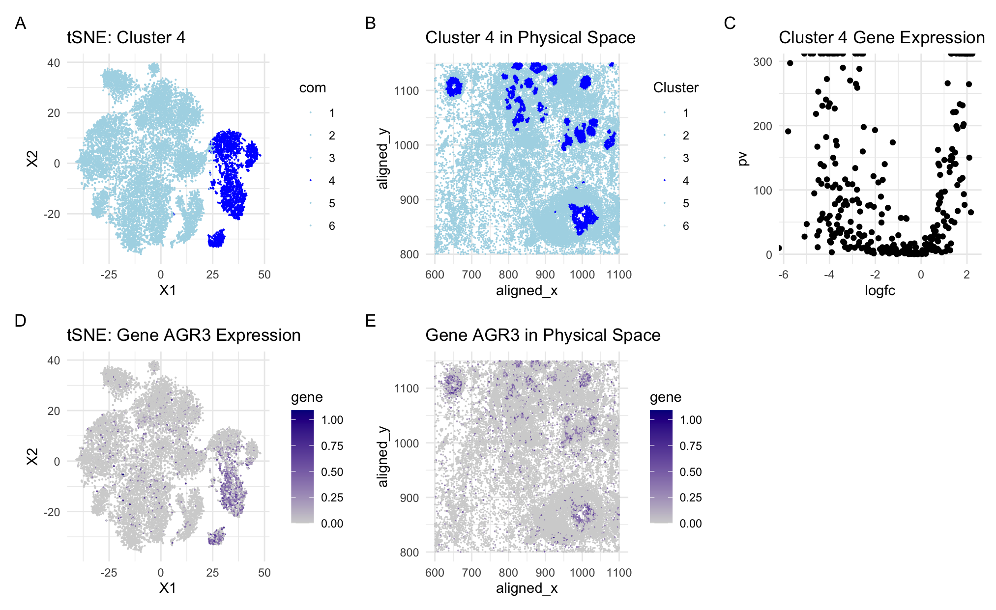
This figure is an analysis of AGR3 expression within a specific cluster and its spatial distribution across the tissue sample. The plots show clustering into groups of 6 with cluster 4 as the cluster of interest and AGR3 as the gene of interest. Both spatial and tSNE visualizations are shown. (A) A tSNE plot illustrating how the cells are clustered and highlighting cluster 4 with dark blue. Cluster 4 is clearly separate from the other cell types. (B) A mapping of cluster 4 cells onto the physical space to illustrate their spatial orientation in the tissue sample. Cluster 4 is encoded in dark blue and these cells are found primarily in the tighter groupings of cells within the tissue sample. (C) A volcano plot showing the significant differential expression of genes in cluster 4. (D) A tSNE plot illustrating the dispersion of cells expressing AGR3 throughout the clusters. The highest levels of expression are the darkest purple and these cells are primarily found in cluster 4. There are a few spots of dark purple scattered throughout the other clusters as well, but the highest gene expression of AGR3 is found in cluster 4. (E) A mapping of AGR3 expression onto the physical space showing levels of AGR3 expression in the different areas of tissue. The darker purple indicates higher gene expression and is primarily found in areas of tighter cell groupings in the tissue.
Conclusion
Based on outside research, AGR3 is highly expressed in breast glandular cells (2). Since AGR3 was the most expressed gene in cluster 4, this makes it likely that cluster 4 is composed primarily of breast glandular cells. Additionally, AGR3 expression has been found to play an important part in estrogen mediated cell proliferation in particular cancer cells with upregulation of the gene indicating an oncogenic state and downregulation of the gene posing a potential therapeutic avenue for certain types of breast cancer (1). Since this gene is associated with breast cancer, it is logical that when examining the spatial representation of the cluster and gene expression, the gene is found to be most expressed in the areas of highest cell density. While this may be a natural occurrence involving gland tissues, it is also possible that is is indicative of cancerous cell behavior.
References
[1] https://www.ncbi.nlm.nih.gov/pmc/articles/PMC7377037/ [2] https://www.proteinatlas.org/ENSG00000173467-AGR3
# code credit to the class notes this past week

# libraries
library(ggplot2)
library(Rtsne)
library(patchwork)

# read in the data
data = read.csv('/Users/Kyra_1/Documents/College/Junior/Spring/Genomic_Data_Visualization/Homework_1/pikachu.csv.gz', row.names = 1)
data[1:5, 1:10]
pos = data[, 4:5]
gexp = data[6:ncol(data)]

# normalize
gexpnorm = log10(gexp/rowSums(gexp) * mean(rowSums(gexp))+1)

# dimensionality reduction: PCA
pcs = prcomp(gexpnorm)
plot(pcs$sdev[1:100])
## most variation is captured by about 20 pcs

# RTSNE
emb = Rtsne(pcs$x[, 1:20])$Y

# kmeans clustering
com = as.factor(kmeans(gexpnorm, centers = 6)$cluster)

# CLUSTER 4
# cluster of interest in reduced space
p1 = ggplot(data.frame(emb,com)) + geom_point(aes(x = X1, y = X2, col = com), size = 0.01)+
  scale_color_manual(values = c("lightblue", "lightblue", "lightblue", "blue", "lightblue", "lightblue"))+
  labs(title = "tSNE: Cluster 4")+
  theme_minimal()

# cluster of interest in physical space
p2 = ggplot(data.frame(pos, Cluster = com)) +
  geom_point(aes(x=aligned_x, y = aligned_y, col = Cluster), size = 0.01)+
  scale_color_manual(values = c("lightblue", "lightblue", "lightblue", "blue", "lightblue", "lightblue"))+
  labs(title = "Cluster 4 in Physical Space")+ theme_minimal()

# volcano plots to visualize differentially expressed genes in the cluster of interest
pv = sapply(colnames(gexp), function(i){
  wilcox.test(gexp[com ==4, i], gexp[com != 1, i])$p.val
})

logfc = sapply(colnames(gexp), function(i){
  ## if this mean is exactly 1, then the means are equal across the population
  log2(mean(gexp[com == 4, i])/mean(gexp[com != 1, i]))
})

p3 = ggplot(data.frame(pv = -log10(pv), logfc))+ geom_point(aes(x = logfc, y = pv))+
  labs(title = "Cluster 4 Gene Expression")+ theme_minimal()

# picking a gene:
# find the most differentially expressed gene in each cluster
results2 <- sapply(1:6, function(i){
  print(i)
  results = sapply(colnames(gexpnorm), function(g){
    wilcox.test(gexpnorm[com == i, g],
                gexpnorm[com != i, g],
                alternative = "greater")$p.val
  })
  topgene = names(head(sort(results, decreasing= F))[1])
  print(topgene)
  return(topgene)
})

# 'AGR3' is the most expressed gene in the fourth cluster
# pick a cluster of interest: CLUSTER 4
g = 'AGR3'
gexpnorm[com == 4, g]
gexpnorm[com != 4, g]
par(mfrow=c(2,1))
hist(gexpnorm[com == 4, g])
hist(gexpnorm[com != 4, g])

# run a t-test
t.test(gexpnorm[com == 4, g], gexpnorm[com != 4, g], alternative = "two.sided")$p.val

# visualizing the gene in reduced dimensional space
p4 = ggplot(data.frame(emb, gene = gexpnorm[, 'AGR3'])) +
  geom_point(aes(x = X1, y = X2, col = gene), size = 0.01)+
  scale_color_gradient2(high = 'darkblue', mid = 'lightgrey', low = 'lightblue')+
  labs(title = "tSNE: Gene AGR3 Expression")+ theme_minimal()

# visualizing the gene in space
## need to modify the data frame still
p5 = ggplot(data.frame(pos, gene = gexpnorm[, 'AGR3'])) +
  geom_point(aes(x=aligned_x, y = aligned_y, col = gene), size = 0.01)+
  scale_color_gradient2(high = 'darkblue', mid = 'lightgrey', low = 'lightblue')+
  labs(title = "Gene AGR3 in Physical Space")+ theme_minimal()


# stitch the graphs together using patchwork
p1 + p2 + p3 + p4 + p5 + plot_annotation(tag_levels = 'A')